Scalable sequences – size check

Motivation

In recent times I speculate where and when to use scalable sequences. Especially if it makes sense to use them in general for sequence driven ID columns of larger tables. I know this sounds a bit like an early sign of CTD (compulsive tuning disorder), but at least I’m aware of it.

Scalable sequences offer a performance benefit in certain special situations (hot block, index contention). This post is not about those benefits.

I assume the reader has a basic understanding what a scalable sequence is. If not, check out this older post of mine: All about sequences .

A scalable sequence provides larger numeric values than a normal sequence does.

A normal sequence => 3
A scalable sequence => 10176700000003

Here I only analyze and test the effects of those bigger numbers, especially for indexes.

Side note: The first 3 digits of the scalable sequence are the instance number + 100. The second 3 digits are the session id. The remainder is the normal sequence value. Different sessions provide different numbers and by this the sequence numbers are not monotonously increasing anymore. At least not when looking at multiple sessions. Which also means inserts are done all over the index and not only on the right hand side of the index.

Bigger numbers need more storage

The number 3 needs 2 bytes, the number 10176700000003 needs 8 bytes of storage. Use the DUMP function to measure it. Values provided by scalable sequences might use up to 18 bytes of storage.

This effects multiple areas, table segment size but also indexes tend to be bigger. We can safely assume the sequences are used to provide values for ID columns which are almost always supported by an unique index. But there are also foreign key columns using those numbers and there the index will not be unique for similar ID values.

Because values are bigger less index references fit into a single index block – meaning we need more index blocks. Here I focus explictly on the size of indexes and not on the size of columns. I believe that a few additional bytes for a whole table row is usually not relevant. In case of an index however the whole row is that single value plus references (index branch block) or rowids (index leaf block).

For comparison reasons I also check the size of an reverse key index since they were used in the past to combat index contention issues. Scalable sequences are the new kid in town that should replace reverse key indexes.

So let’s measure it.

Testscript 1 – single session insert

First we create a table with 3 number columns. Then we create a normal and a scalable sequence that provide some values. We add two normal and a reverse key index on those 3 columns and populate the table with values originating from the sequences.

------------------------------------------------------------------------------- Scenario: Test index size
--------------------------------------------------------------------------------
-- create a table with two columns files with IDs
create table test_sequence_effects 
  (id_normal number, 
   id_scalable number,
   id_reverse number);

-- create a normal and a scalable sequence
create sequence test_sequence_normal;
create sequence test_sequence_scale scale;

-- create 3 indexes
create index test_sequence_normal_ix on test_sequence_effects(id_normal); 
create index test_sequence_scale_ix on test_sequence_effects(id_scalable);
create index test_sequence_reverse_ix on test_sequence_effects(id_reverse) reverse ;

-- insert 1 million datapoints
insert into test_sequence_effects 
select test_sequence_normal.nextval, test_sequence_scale.nextval, test_sequence_normal.nextval 
from dual connect by level <= 1000000;

commit;

-- create statistics
execute dbms_stats.gather_index_stats(user, 'TEST_SEQUENCE_NORMAL_IX',estimate_percent => 100);
execute dbms_stats.gather_index_stats(user, 'TEST_SEQUENCE_SCALE_IX',estimate_percent => 100);
execute dbms_stats.gather_index_stats(user, 'TEST_SEQUENCE_REVERSE_IX',estimate_percent => 100);

result after single session insert

We can have a look at the index statistics and the segment sizes.

-- check index stats
select index_name, blevel, leaf_blocks, distinct_keys, clustering_factor 
from dba_indexes 
where index_name like 'TEST_SEQUENCE_%'; 
INDEX_NAMEBLEVELLEAF_BLOCKSDISTINCT_KEYSCLUSTERING_FACTOR
TEST_SEQUENCE_NORMAL_IX2199910000004271
TEST_SEQUENCE_SCALE_IX2337910000004271
TEST_SEQUENCE_REVERSE_IX 229651000000999996

Now all three indexes still have the same blevel, meaning for a single direct index access the performance should be identical. However when the number of entries increases eventually the ID values created by a scalable sequence might create a new level in the btree before the same happens for IDs from a normal sequence. I tested when this will happen. If you are curious check out the appendix section “blevel3 break point”, but try to guess the value before you check.

-- check index size
select segment_name, segment_type, segment_subtype, blocks, bytes/1024/1024 as size_in_MB
from user_segments
where segment_name like 'TEST_SEQUENCE_%';
SEGMENT_NAMESEGMENT_TYPESEGMENT_SUBTYPEBLOCKSSIZE_IN_MB
TEST_SEQUENCE_EFFECTS TABLE ASSM 4352 34
TEST_SEQUENCE_NORMAL_IX INDEX ASSM 2176 17
TEST_SEQUENCE_REVERSE_IX INDEX ASSM 3072 24
TEST_SEQUENCE_SCALE_IX INDEX ASSM 3584 28
table and index size

The scaleable index in this experiment is 65% larger than the normal index. The cause for this increment can be attributed directly to the bigger numbers that needs to be stored.

We have to keep in mind that the test scenario was run in a single session. In reality multiple sessions will be used to run the insert(s). This is where scalable sequences should give a performance boost, even at the cost of potentially slightly higher storage consumption.

Testscript 2 – parallel inserts from multiple sessions

Ok now repeat the same experiment but using multiple sessions instead of a single session.

I created a code block that repeatetly does single row inserts in blocks of 10 and waits 1 second. This was run in up to 100 parallel sessions using dbms_scheduler jobs until approximately 1 million rows were inserted. The code for this test can be found in the appendix section “Testscript 2 – code”. Because of the 1 sec. pause this will run for some time.

Index stats after parallel inserts

INDEX_NAMEBLEVELLEAF_BLOCKSDISTINCT_KEYSCLUSTERING_FACTOR
TEST_SEQUENCE_NORMAL_IX23649 1000198 943211
TEST_SEQUENCE_SCALE_IX26577 1000198 32329
TEST_SEQUENCE_REVERSE_IX23240 1000198 986633

The number of blocks increased for all indexes. But more importantly we see that the clustering factor for the normal index went through the roof and is now close to the number of rows in the table. Which is bad. It also shows that scalable sequences seem to keep the promise of avoiding index contention and hot blocks, even if this test was not set up to measure any performance implications.

If you want to know more about clustering factor, read appendix section “index clustering factor”.

Side note: There were a few more rows inserted than in the single session approach (0.02%). That was because how the stopping mechanism worked for the parallel jobs. It does not influence the comparison at all.

Index sizes after parallel inserts

SEGMENT_NAMESEGMENT_TYPESEGMENT_SUBTYPEBLOCKSSIZE_IN_MB
TEST_SEQUENCE_EFFECTSTABLEASSM4480 35
TEST_SEQUENCE_NORMAL_IXINDEXASSM3840 30
TEST_SEQUENCE_REVERSE_IXINDEXASSM3328 26
TEST_SEQUENCE_SCALE_IXINDEXASSM6784 53

So the size of a normal index rose from 17 to 30MB (76% increase) and for the scaleable index from 28 to 53MB (83%). The reason for both increaments in size should be because now we see more 50-50 index block splits resulting in a considerable amount of blocks not being full and rarely being reused.

Overall the size didn’t explode, but it is still a noticable amount.

Side note: It is possible to shrink the indexes after such parallel insert sessions, but the effect is not great. Shrink and coalesce really should be considered when frequent deletes are run against the table. Scalable sequences potentially can provide values that might fill some of the gaps created by deletes. An index rebuild is not needed or advisable as long as more inserts are to come.

Conclusion

Values created by scalable sequences are using more storage space than values from normal sequences. For indexes we can expect a growth in index size between 50% and 100% compared to a normal index. The growth is partially because of larger numbers but also because there will be more not yet used space in many of the index blocks (caused by 50-50 index block splits instead of 90-10).

The clustering factor for scalable sequences always is better or equal than any alternative.

For all customers that I work with such an increment in storage size would not be any problem at all, especially if there is a performance improvement.

For me the storage size increase is not an argument against scalable sequences.

Appendix

Testscript 2 – code

--------------------------------------------------------------------------------
-- Scenario: Test index size after parallel inserts
--------------------------------------------------------------------------------
-- cleanup logic
drop table test_sequence_effects purge;
drop sequence test_sequence_normal;
drop sequence test_sequence_scale;

execute dbms_scheduler.drop_program('test_sequence_do_inserts');
begin
 for j in (select job_name from all_scheduler_jobs where job_name like 'TEST_SEQUENCE%') loop
     dbms_scheduler.drop_job(j.job_name);
 end loop;    
end;
/
--------------------------------------------------------------------------------
-- create a table with three columns to be filled with IDs
create table test_sequence_effects 
  (id_normal number, 
   id_scalable number,
   id_reverse number);

-- create a normal and a scalable sequence
create sequence test_sequence_normal;
create sequence test_sequence_scale scale;

-- create 3 indexes
create index test_sequence_normal_ix on test_sequence_effects(id_normal); 
create index test_sequence_scale_ix on test_sequence_effects(id_scalable);
create index test_sequence_reverse_ix on test_sequence_effects(id_reverse) reverse ;

-- insert 1 million datapoints
-- run as 100 parallel scheduled jobs 
-- each job inserts a batch of 10 IDs using single row inserts 
-- each job waits for 10 seconds before the next batch is run
-- each job stops after the max number for the normal ID is reached.

--create a program for dbms_scheduler to be used in jobs later
begin
    DBMS_SCHEDULER.create_program (
    program_name   => 'test_sequence_do_inserts',
    program_type   => 'PLSQL_BLOCK',
    program_action => q'[declare
  last_id number;
  max_id number := 1000000;
  cnt_id number := 0;
  e_stop exception;
  pragma exception_init (e_Stop, -20022);
begin 
  for j in 1..max_id/10 loop
    -- single insert for 10 rows 
    for i in 1..10 loop
        insert into test_sequence_effects 
        values (test_sequence_normal.nextval -- ID_NORMAL
             , test_sequence_scale.nextval  -- ID_SCALABLE
             , test_sequence_normal.nextval -- ID_REVERSE
             )
        returning id_normal into last_id;
        cnt_id := cnt_id + 1;
        if last_id >= max_id then 
          commit;
          raise e_stop;
        end if;   
    end loop;
    commit; 
    -- pause for 1 sec  
    dbms_session.sleep(1);
  end loop;  
exception
 when e_stop then
   -- finish gracefully
   dbms_output.put_line('This session inserted '||to_char(cnt_id)||' rows');
   commit;
end;
]',
    enabled        => TRUE,
    comments       => 'Insert 10 rows, 1 sec pause.');


   -- activate the program. This does not run the logic yet.
   DBMS_SCHEDULER.enable (name => 'test_sequence_do_inserts');

end;
/

-- create multiple jobs
begin 
  for j in 1..100 loop
     dbms_scheduler.create_job
     (job_name      => 'test_sequence_do_inserts_job'||to_char(j,'FM000'),
      program_name  => 'test_sequence_do_inserts',
      start_date => systimestamp,
      enabled => true);

     dbms_scheduler.run_job (job_name => 'test_sequence_do_inserts_job'||to_char(j,'FM000'),
                              use_current_session => false);
   end loop;
end;
/


After executing this script the scheduled job runs for quite some time.

We can check the number of rows in the table to see if it is finished.

select max(id_normal) last_value,count(*) row_count from test_sequence_effects;

other interesting selects to monitor the scheduled jobs

-- check scheduler jobs
select * from all_scheduler_programs;
select * from all_scheduler_jobs where job_name like 'TEST_SEQUENCE%';
select * from all_scheduler_running_jobs where job_name like 'TEST_SEQUENCE%';
select * from all_scheduler_job_log where job_name like 'TEST_SEQUENCE%';
select * from all_scheduler_job_run_details where job_name like 'TEST_SEQUENCE%';

And of cause the statistics need to be gathered

-- compute statistics for all indexes
execute dbms_stats.gather_index_stats(user, 'TEST_SEQUENCE_NORMAL_IX',estimate_percent => 100);
execute dbms_stats.gather_index_stats(user, 'TEST_SEQUENCE_SCALE_IX',estimate_percent => 100);
execute dbms_stats.gather_index_stats(user, 'TEST_SEQUENCE_REVERSE_IX',estimate_percent => 100);

Index clustering factor

What is the clustering factor of an index? Essentially it tells us how good the index and the table data match. How many table blocks need to be read if each block is accessed via the index? The value itself needs to be compared with the number of blocks (min value) and rows (max value) in the table.

Here are some links that might improve your understanding of the clustering factor:

http://dbaparadise.com/2018/05/what-is-index-clustering-factor/

Ask Tom: https://asktom.oracle.com/pls/apex/f?p=100:11:0::::P11_QUESTION_ID:1032431852141

David Fitzjarrell in detail about the clustering factor and Oracles calculation of it

Blevel 3 break point

I run some further tests to see when the index based upon a scalable sequence will reach blevel3.

For a single session insert, blevel 3 was reached after approximately 38 million inserts.

INDEX_NAME                  BLEVEL LEAF_BLOCKS DISTINCT_KEYS CLUSTERING_FACTOR
--------------------------- ------ ----------- ------------- -----------------
TEST_SEQUENCE_NORMAL_IX          2       81148      38200000            173362
TEST_SEQUENCE_REVERSE_IX         2      125912      38200000          38199995
TEST_SEQUENCE_SCALE_IX           3      129055      38200000            173362

For multiple sessions the same amount of blocks/leaf blocks should be reached earlier. However the distribution would be considerably more even. Both effects will partially cancel each other out. So far I didn’t measure it.

dbms_stats quickie: show global and table preferences

Introduction

To gather statistics for a schema or a table there is the dbms_stats package. Either we call it manually or the automatic statistic gathering (scheduled) job is used.

We can provide many settings for the statistic gathering job as a parameter during the gather call. For parameters that we do not explicitly set, preferences are used. Either on a global or on individual table level.

Since there are many preferences this article has some SQL statements that help to check how the current dbms_stats preferences are.

Table preferences overrule the global preferences. And preferences set by calling gather_..._stats overrule the table preferences. However it is possible to override this last rule by setting the preference_overrides_parameter to true. In that case the table preferences overrule the gather_..._stats parameters.
see https://docs.oracle.com/en/database/oracle/oracle-database/21/tgsql/options-for-optimizer-statistics-gathering.html#GUID-E616363F-0A7B-4D4D-9384-63934DB69F7D

show global preferences

Script to show the global preferences. Note that the parameter autostats_target can not be set on table level, because it directly influences the area of work for the auto stats gathering job.

set linesize 250
set pagesize 100
column preference_name format a30
column preference_value format a50

-- global preferences
with preflist (preference_name,global_only)
as (select 'APPROXIMATE_NDV_ALGORITHM',0 from dual union all
    select 'AUTO_STAT_EXTENSIONS'     ,0 from dual union all
    select 'AUTO_TASK_STATUS'         ,0 from dual union all
    select 'AUTO_TASK_MAX_RUN_TIME'   ,0 from dual union all
    select 'AUTO_TASK_INTERVAL'       ,0 from dual union all
    select 'AUTOSTATS_TARGET'         ,1 from dual union all
    select 'CASCADE'                  ,0 from dual union all
    select 'CONCURRENT'               ,0 from dual union all
    select 'DEGREE'                   ,0 from dual union all
    select 'ESTIMATE_PERCENT'         ,0 from dual union all
    select 'GLOBAL_TEMP_TABLE_STATS'  ,0 from dual union all
    select 'GRANULARITY'              ,0 from dual union all
    select 'INCREMENTAL'              ,0 from dual union all
    select 'INCREMENTAL_STALENESS'    ,0 from dual union all
    select 'INCREMENTAL_LEVEL'        ,0 from dual union all
    select 'METHOD_OPT'               ,0 from dual union all
    select 'NO_INVALIDATE'            ,0 from dual union all
    select 'OPTIONS'                  ,0 from dual union all
    select 'PREFERENCE_OVERRIDES_PARAMETER',0 from dual union all
    select 'PUBLISH'                  ,0 from dual union all
    select 'STALE_PERCENT'            ,0 from dual union all
    select 'STAT_CATEGORY'            ,0 from dual union all
    select 'TABLE_CACHED_BLOCKS'      ,0 from dual union all
    select 'WAIT_TIME_TO_UPDATE_STATS',0 from dual )
select preference_name, 
       sys.dbms_stats.get_prefs(preference_name) as preference_value,
       global_only
from preflist;

And the result might look like this

PREFERENCE_NAMEPREFERENCE_VALUE
APPROXIMATE_NDV_ALGORITHMHYPERLOGLOG
AUTO_STAT_EXTENSIONSOFF
AUTO_TASK_STATUSOFF
AUTO_TASK_MAX_RUN_TIME3600
AUTO_TASK_INTERVAL900
AUTOSTATS_TARGETORACLE
CASCADEDBMS_STATS.AUTO_CASCADE
CONCURRENTOFF
DEGREENULL
ESTIMATE_PERCENTDBMS_STATS.AUTO_SAMPLE_SIZE
GLOBAL_TEMP_TABLE_STATSSESSION
GRANULARITYAUTO
INCREMENTALFALSE
INCREMENTAL_STALENESSNULL
INCREMENTAL_LEVELPARTITION
METHOD_OPTFOR ALL COLUMNS SIZE AUTO
NO_INVALIDATEDBMS_STATS.AUTO_INVALIDATE
OPTIONSGATHER
PREFERENCE_OVERRIDES_PARAMETERFALSE
PUBLISHTRUE
STALE_PERCENT10
STAT_CATEGORYOBJECT_STATS, REALTIME_STATS
TABLE_CACHED_BLOCKS1
WAIT_TIME_TO_UPDATE_STATS15
global preferences for dbms_stats

Show table preferences

And here is how to show the preferences for a single (or a few) table(s) and compare them to the global preferences. Add your table names to the list of tables in the tabs subquery.

-- table preferences
with tabs (owner, table_name)
  as (select user , 'MYTABLE1' from dual union all
      select 'STAGE' , 'MYTABLE2' from dual union all
      select 'STAGE' , 'MYTABLE' from dual
      )
, preflist (preference_name, global_only)
as (select 'APPROXIMATE_NDV_ALGORITHM',0 from dual union all
    select 'AUTO_STAT_EXTENSIONS'     ,0 from dual union all
    select 'AUTO_TASK_STATUS'         ,0 from dual union all
    select 'AUTO_TASK_MAX_RUN_TIME'   ,0 from dual union all
    select 'AUTO_TASK_INTERVAL'       ,0 from dual union all
    select 'AUTOSTATS_TARGET'         ,1 from dual union all
    select 'CASCADE'                  ,0 from dual union all
    select 'CONCURRENT'               ,0 from dual union all
    select 'DEGREE'                   ,0 from dual union all
    select 'ESTIMATE_PERCENT'         ,0 from dual union all
    select 'GLOBAL_TEMP_TABLE_STATS'  ,0 from dual union all
    select 'GRANULARITY'              ,0 from dual union all
    select 'INCREMENTAL'              ,0 from dual union all
    select 'INCREMENTAL_STALENESS'    ,0 from dual union all
    select 'INCREMENTAL_LEVEL'        ,0 from dual union all
    select 'METHOD_OPT'               ,0 from dual union all
    select 'NO_INVALIDATE'            ,0 from dual union all
    select 'OPTIONS'                  ,0 from dual union all
    select 'PREFERENCE_OVERRIDES_PARAMETER',0 from dual union all
    select 'PUBLISH'                  ,0 from dual union all
    select 'STALE_PERCENT'            ,0 from dual union all
    select 'STAT_CATEGORY'            ,0 from dual union all
    select 'TABLE_CACHED_BLOCKS'      ,0 from dual union all
    select 'WAIT_TIME_TO_UPDATE_STATS',0 from dual
    )
,tabprefs as (select t.owner, t.table_name, preference_name, 
       sys.dbms_stats.get_prefs(preference_name,null,null) as preference_global,
       case when global_only=0 
            then sys.dbms_stats.get_prefs(preference_name,t.owner,t.table_name) 
       end as preference_table,
       global_only
       from preflist 
       cross join tabs t
)
select p.*, 
       case when global_only=1 then null
            when preference_global=preference_table then 'FALSE' 
             else 'TRUE' 
             end as individual_table_pref
from tabprefs p
;

The select gives a comparison between the preferences on global and on table level.

OWNERTABLE_NAMEPREFERENCE_NAMEPREFERENCE_GLOBALPREFERENCE_TABLEGLOBAL_ONLYINDIVIDUAL_TABLE_PREF
SVENMYTABLE1APPROXIMATE_NDV_ALGORITHMHYPERLOGLOGHYPERLOGLOG0FALSE
SVENMYTABLE1AUTO_STAT_EXTENSIONSOFFOFF0FALSE
SVENMYTABLE1AUTO_TASK_STATUSOFFOFF0FALSE
SVENMYTABLE1AUTO_TASK_MAX_RUN_TIME360036000FALSE
SVENMYTABLE1AUTO_TASK_INTERVAL9009000FALSE
SVENMYTABLE1AUTOSTATS_TARGETORACLE1
SVENMYTABLE1CASCADEDBMS_STATS.AUTO_CASCADEDBMS_STATS.AUTO_CASCADE0FALSE
SVENMYTABLE1CONCURRENTOFFOFF0FALSE
SVENMYTABLE1DEGREENULLNULL0FALSE
SVENMYTABLE1ESTIMATE_PERCENTDBMS_STATS.AUTO_SAMPLE_SIZEDBMS_STATS.AUTO_SAMPLE_SIZE0FALSE
SVENMYTABLE1GLOBAL_TEMP_TABLE_STATSSESSIONSESSION0FALSE
SVENMYTABLE1GRANULARITYAUTOAUTO0FALSE
SVENMYTABLE1INCREMENTALFALSETRUE0TRUE
SVENMYTABLE1INCREMENTAL_STALENESSNULLNULL0FALSE
SVENMYTABLE1INCREMENTAL_LEVELPARTITIONPARTITION0FALSE
SVENMYTABLE1METHOD_OPTFOR ALL COLUMNS SIZE AUTOFOR ALL COLUMNS SIZE AUTO0FALSE
SVENMYTABLE1NO_INVALIDATEDBMS_STATS.AUTO_INVALIDATEDBMS_STATS.AUTO_INVALIDATE0FALSE
SVENMYTABLE1OPTIONSGATHERGATHER0FALSE
SVENMYTABLE1PREFERENCE_OVERRIDES_PARAMETERFALSEFALSE0FALSE
SVENMYTABLE1PUBLISHTRUETRUE0FALSE
SVENMYTABLE1STALE_PERCENT10100FALSE
SVENMYTABLE1STAT_CATEGORYOBJECT_STATS, REALTIME_STATSOBJECT_STATS, REALTIME_STATS0FALSE
SVENMYTABLE1TABLE_CACHED_BLOCKS110FALSE
SVENMYTABLE1WAIT_TIME_TO_UPDATE_STATS15150FALSE
table preferences for dbms_stats

The last column INDIVIDUAL_TABLE_PREF indicates whether the global setting was changed on table level or not. But take it with a grain of salt. Some preferences might have additional restrictions, like the INCREMENTAL_LEVEL can be set to PARTITION only if the table is actually partitioned. Otherwise the default for the table will be TABLE, even if the global setting differs.

Show all changed preferences on table level for a schema

And finally here is a statement that goes through all the tables in one (or several schemas) and finds settings where the global and the table preference differs. For each preference value combination it lists the number of table and the table names.

In the tabs subquery list all the schemas you want to be checked.

-- All tables with a non default setting
with tabs
  as (select owner, table_name, partitioned 
      from dba_tables
      where owner in (user,'STAGE')
      )
,preflist (preference_name, global_only)
as (select 'APPROXIMATE_NDV_ALGORITHM',0 from dual union all
    select 'AUTO_STAT_EXTENSIONS'     ,0 from dual union all
    select 'AUTO_TASK_STATUS'         ,0 from dual union all
    select 'AUTO_TASK_MAX_RUN_TIME'   ,0 from dual union all
    select 'AUTO_TASK_INTERVAL'       ,0 from dual union all
    select 'AUTOSTATS_TARGET'         ,1 from dual union all
    select 'CASCADE'                  ,0 from dual union all
    select 'CONCURRENT'               ,0 from dual union all
    select 'DEGREE'                   ,0 from dual union all
    select 'ESTIMATE_PERCENT'         ,0 from dual union all
    select 'GLOBAL_TEMP_TABLE_STATS'  ,0 from dual union all
    select 'GRANULARITY'              ,0 from dual union all
    select 'INCREMENTAL'              ,0 from dual union all
    select 'INCREMENTAL_STALENESS'    ,0 from dual union all
    select 'INCREMENTAL_LEVEL'        ,0 from dual union all
    select 'METHOD_OPT'               ,0 from dual union all
    select 'NO_INVALIDATE'            ,0 from dual union all
    select 'OPTIONS'                  ,0 from dual union all
    select 'PREFERENCE_OVERRIDES_PARAMETER',0 from dual union all
    select 'PUBLISH'                  ,0 from dual union all
    select 'STALE_PERCENT'            ,0 from dual union all
    select 'STAT_CATEGORY'            ,0 from dual union all
    select 'TABLE_CACHED_BLOCKS'      ,0 from dual union all
    select 'WAIT_TIME_TO_UPDATE_STATS',0 from dual
    )
,tabprefs as (select t.owner, t.table_name, t.partitioned, 
       preference_name, global_only,
       sys.dbms_stats.get_prefs(preference_name,null,null) as preference_global,
       case when global_only=0 then sys.dbms_stats.get_prefs(preference_name,t.owner,t.table_name) end as preference_table
       from preflist 
       cross join tabs t
)
select preference_name, preference_global, preference_table, listagg(owner||'.'||table_name,',' on overflow truncate without count) within group (order by owner, table_name) tables, count(*) table#
from tabprefs p
where global_only=0
and preference_global!=preference_table 
-- Special case: incremental_level can only be TABLE for non partitioned tables, even if default is different.
and not (preference_name='INCREMENTAL_LEVEL' and partitioned='NO' and preference_table='TABLE' and preference_global='PARTITION')
group by preference_name, preference_global, preference_table
order by preference_name, preference_global, preference_table;

Note that there is some special consideration for the previously mentioned INCREMENTAL_LEVEL preference.

PREFERENCE_NAMEPREFERENCE_GLOBALPREFERENCE_TABLETABLESTABLE#
INCREMENTALFALSETRUESVEN.ANTRAG_BESTAND,SVEN.ANTRAG_DETAIL,SVEN.ANTRAG_PRODUKT,…203
tables with individual preferences

So in this case there were 203 tables (not all names shown) where the INCREMENTAL preference on table level was set to TRUE compared to the global setting of FALSE. This indicates that the global preference was changed, after most of the tables had been created.

Conclusion

It is hard to remember all the different settings that do influence stats gathering. Especially in cases where we wonder, why the settings did not seem to work as expected, it helps to check all the preferences on each level.

secret oracle db features

10 “secret” Oracle DB features you might not know

“Secret” here means either not documented or hidden in the documentation so deep that is is almost impossible to find.

1 – restart sequence

We can use a single ddl statement to reset a sequence. Works from 12.2 onwards.

alter sequence mySeq restart start with 115;

It is also possible to use this to reset an identity column!

alter table myTable
modify ID generated always as identity 
       restart start with 115;

This is not (yet) documented.

2 – hidden format options

We can display a negative number in round brackets using the “pt” format option. Which is not in the list of format options in the SQL reference.

select to_char(-10,'fm9990pt') from dual;
(10)

documented is the “pr” option which uses angle brackets

select to_char(-10,'fm9990pr') from dual;
<10>

See also this ODC thread.

This is documented, but not in the SQL Reference but in some OBI Publisher documentation.

3 – sample (x,y)

The SAMPLE clause is documented. It is part of the query table expression clause. Not documented is the second secret parameter y.

sample clause
https://docs.oracle.com/en/database/oracle/oracle-database/19/sqlrf/img_text/sample_clause.html

The sample clause allows us to get a portion (a sample) of the tables data.

select * 
from employees SAMPLE(20); 

This returns 20 percent of the employees.

There is a ROW mode and a BLOCK mode. In BLOCK mode 20% of the blocks are returned, instead of 20% of the rows.

The sample clause has a second undocumented parameter.

select *
from employees SAMPLE(20, 0.5);

This also returns 20%. So far no obvious difference…

Jonathan Lewis mentioned that this second parameter is the number of consecutive groups/rows during row or block sampling. It was introduced during changes for the SAMPLE clause in 10g.

My non-representative tests showed that setting this parameter to 1 during block sampling makes sure we get results. Otherwise we frequently get blocks from the tables tablespace that are not filled with data. This seems to depend on the data distribution.

So… if a query like the following returns 0…

-- how many rows are in 1% of the blocks?
select count(*)
from employees SAMPLE BLOCK (1);
0

… then you can set the second parameter to 1 to be sure to get some data.

-- how many rows are in 1% of the blocks?
select count(*)
from employees SAMPLE BLOCK (1, 1);
110

Use at your own risk!

See also this ODC thread.

4 – Exadata test parameter

Warning! This is only for testing purposes! It can potentially destroy your database.

alter system set "_exadata_feature_on"=true scope=spfile;
shutdown immediate;
startup;

Using this parameter we can test some of the newest options which are available only on exadata/cloud, like automated indexing.

5 – sequence cache is not lost during graceful database shutdown

Shutdown normal|immediate|transactional will not loose the sequence cache. Instead the next value will be used and set as last_number. Only a shutdown abort will loose the cache.

This was documented somewhere but I am not able to find it anymore. it might be that only older versions of the oracle docs still have this information.

To confirm it, I tested it. It works in SE and EE. It will probably not work in the same way on a RAC – because there is a separate cache for each instance.

There is an indirect mention of the behaviour in the 11g admin guide.

The database might skip sequence numbers if you choose to cache a set of sequence numbers. For example, when an instance abnormally shuts down (for example, when an instance failure occurs or a SHUTDOWN ABORT statement is issued), sequence numbers that have been cached but not used are lost. Also, sequence numbers that have been used but not saved are lost as well. The database might also skip cached sequence numbers after an export and import. See Oracle Database Utilities for details.

So a shutdown abort will loose the sequence cache. All other “organized” shutdowns will keep the cache intact.

The problem is that most DBAs seem way too keen on doing a shutdown abort. So loosing the sequence cache looks like the default behaviour, although it is not.

6 – reorder columns

We can change the logical column order by setting them invisible and making them visible again. This can be used to reorder columns in the column list. Important to understand is that the table is not physically changed, only the data dictionary entry is manipulated.

If we want to reorder columns physically, maybe to improve data compression, then this is not the way to do it.

example

create table t (col1 number, col2 number);
Table T created.

desc t;
Name Null? Type   
---- ----- ------ 
COL1       NUMBER 
COL2       NUMBER 

/* make the first column invisible */
alter table t modify col1 invisible;
Table T altered.

desc t;
Name Null? Type   
---- ----- ------ 
COL2       NUMBER 

/* make the first column visible again */
alter table t modify col1 visible;
Table T altered.

desc t;
Name Null? Type   
---- ----- ------ 
COL2       NUMBER 
COL1       NUMBER 

/* the column order is now reversed */

To physically reorder a table we need to export/import it, use dbms_redefinition or move the table.

Side note: The describe command in SQL*plus (and SQL Developer) will not show invisible columns. You can change that by setting the documented SQL*PLUS parameter COLINVISIBLE.

SET COLINVISIBLE ON

desc t;
Name             Null? Type   
---------------- ----- ------ 
COL2                   NUMBER 
COL1 (INVISIBLE)       NUMBER 

7 – object type “NON-EXISTENT”

Namespaces are used to avoid naming clashes between objects of different types. Among others the namespace 1 includes the object types table, view and function. So we can not have a table with the same name as a view or as a function.

There is a special object type in namespace 1 that is called “NON-EXISTENT”. This object type is used to mark dropped objects under edition based redefinition (EBR).

demo

Assuming 3 editions: ORA$BASE => CHILD1 => CHILD2

-- switch to base edition (ORA$BASE)
ALTER SESSION SET EDITION="ORA$BASE";

Adding editionable code in the parent edition ORA$BASE.

-- create a new function in base (EDITIONABLE is the default)
create function test_editions return varchar2
as 
begin
  return 'Base';
end;
/

Test the function in the child edition. It is usable. Although we didn’t create it there yet.

-- switch to child edition (CHILD1)
ALTER SESSION SET EDITION="CHILD1";

-- test function
select test_editions from dual;
TEST_EDITIONS
Base
function is functioning…

Now remove the function from the child edition, but not from the parent.

-- drop code
drop function test_editions;

-- test function again
select test_editions from dual;

ORA-00904: “TEST_EDITIONS”: invalid identifier

This error message was expected. The function was removed. No real object with the name “TEST_EDITIONS” exists (in namespace 1) in the edition CHILD1.
Just to be on the safe side, double check in parent edition:

-- switch back to base and test function
ALTER SESSION SET EDITION="ORA$BASE";
select test_editions from dual;
TEST_EDITIONS
Base
function still functioning in BASE

This is also the result that was expected. The function still works in the parent edition.

What does the data dictionary say? A special view user_objects_ae shows the objects from all editions (_ae):

-- Check dictionary
select object_name, edition_name, object_type, namespace, editionable, status
from user_objects_ae
where object_name = 'TEST_EDITIONS';
OBJECT_NAMEEDITION_NAMEOBJECT_TYPENAMESPACEEDITIONABLESTATUS
TEST_EDITIONSORA$BASEFUNCTION1YVALID
TEST_EDITIONSCHILD1NON-EXISTENT1VALID
TEST_EDITIONSCHILD2FUNCTION1YINVALID

We see that in edition “CHILD1” the object type of the function now is “NON-EXISTENT”. This is important, otherwise the database would not know to return the ORA-00904 error message when it searches for this object.

If the whole row would not exist, then the object in edition CHILD1 would be inherited from the parent edition ORA$BASE. This was the data situation before the function was actualized in CHILD1.

Even after we drop the function from all editions, then the dictionary will still show the NON-EXISTENT entries.

A side note/warning:

The status of the function in the second child edition CHILD2 is invalid after running the sample code. This dictionary entry was created, when the function was dropped in CHILD1.

This is because this function was never compiled in CHILD2. That means the code never was actualized there. And when we drop the code from all parent editions, then in CHILD2 any try to compile the code will not give an error, but the status will remain invalid.

This is why it is strongly recommended to recompile all editionable objects after some code changes, but especially after deletes/drops. Each recompile breaks the relationship to the parent and actualizes the code. So code changes in the parent will not propagate to the child anymore after it was recompiled at least once in the child.

8 – connect / as sysdba to PDB

Using a bequeath connection we can login to an Oracle database without a username and a password. This only works directly on the server using an os account that has enhanced privileges (part of the oradba group). To do so the ORACLE_SID environment variable needs to be set. However this connects only to the CDB.

It is possible to do the same using the undocumented environment variable ORACLE_PDB_SID to do the same against a PDB.

Mike Dietrich has posted a nice blog post about it: https://mikedietrichde.com/2020/05/07/can-you-connect-as-sysdba-without-password-into-a-pdb-directly/

export ORACLE_SID=MYCDB
export ORACLE_PDB_SID=MYPDB

$ sqlplus / as sysdba
SQL> show con_name

CON_NAME
------------------------------
MYPDB

9 – print boolean values to serveroutput

There is an undocumented utility package sys.dbms_metadata_util that has a couple of interesting helper methods.

For example put_bool can be used to print boolean variables to serveroutput (using dbms_output).

-- print boolean values to dbms_output
set serveroutput on
begin
  sys.dbms_metadata_util.put_bool('This is ', TRUE);
  sys.dbms_metadata_util.put_bool('This is ', FALSE);
  sys.dbms_metadata_util.put_bool('This is ', NULL);
end;
/
META:13:17:57.489: This is TRUE
META:13:17:57.489: This is FALSE

PL/SQL procedure successfully completed.

There are also several other interesting functions in this package. For example a way to convert dictionary column values of type LONG into a CLOB variable.

v_view_source := sys.dbms_metadata_util.long2clob(10000,'USER_SOURCE','TEXT',25) ;

10 – undo_sql

There is a way to create the opposite of an SQL DML statement. For an insert we get a delete, for a delete we get an insert with the deleted column values and for an update we get an update with the previous values.

This is documented, but not many people know about. It is part of the flashback logic and more specifically the flashback transaction query.

Using Oracle Flashback Transaction Query

Use Oracle Flashback Transaction Query to retrieve metadata and historical data for a given transaction or for all transactions in a given time interval. Oracle Flashback Transaction Query queries the static data dictionary view FLASHBACK_TRANSACTION_QUERY, whose columns are described in Oracle Database Reference.

The column UNDO_SQL shows the SQL code that is the logical opposite of the DML operation performed by the transaction. You can usually use this code to reverse the logical steps taken during the transaction. However, there are cases where the UNDO_SQL code is not the exact opposite of the original transaction. For example, a UNDO_SQL INSERT operation might not insert a row back in a table at the same ROWID from which it was deleted.

Some security researchers (Alexander Kornbrust at DOAG 2019 – page 74) believe this poses an security risk, especially because it would allow us to find out about column values that are redacted. There are several ways to circumvent data redaction, and Oracle itself states that this feature is not ment as a high secure implementation (see Security Guidelines). So I don’t see that of a high risk. Using undo_sql to circumvent data redaction is the most complex hack I have seen so far – there are way easier methods.


Still an interesting feature. Here is an example.
It needs a lot of non default settings to make it work.

example

Using the HR demo schema to test this.

First some steps to enable supplemental logging which is needed for undo_sql to work.

-- preparations as DBA in the CDB
select * from dba_pdbs;
alter session set container = CDB$ROOT;
ALTER DATABASE ADD SUPPLEMENTAL LOG DATA;
alter session set container = ORCL;
-- and as HR
ALTER TABLE HR.EMPLOYEES ADD SUPPLEMENTAL LOG DATA (ALL) COLUMNS;

Now we can do some changes.

-- as HR user
select * from hr.employees;

update hr.employees
set last_name = '--secret--'
where first_name = 'Randall';
2 rows updated.
delete from hr.employees
where first_name = 'Randall';
2 rows deleted.

Don’t commit or rollback yet. Simply change to another session/account.

-- as DBA
select undo_sql
from FLASHBACK_TRANSACTION_QUERY
where table_name='EMPLOYEES';

Result:

insert into "HR"."EMPLOYEES"("EMPLOYEE_ID","FIRST_NAME","LAST_NAME","EMAIL","PHONE_NUMBER","HIRE_DATE","JOB_ID","SALARY","COMMISSION_PCT","MANAGER_ID","DEPARTMENT_ID") values ('191','Randall','--secret--','RPERKINS','650.505.4876',TO_DATE('19-DEC-99', 'DD-MON-RR'),'SH_CLERK','2500',NULL,'122','50');
insert into "HR"."EMPLOYEES"("EMPLOYEE_ID","FIRST_NAME","LAST_NAME","EMAIL","PHONE_NUMBER","HIRE_DATE","JOB_ID","SALARY","COMMISSION_PCT","MANAGER_ID","DEPARTMENT_ID") values ('143','Randall','--secret--','RMATOS','650.121.2874',TO_DATE('15-MAR-98', 'DD-MON-RR'),'ST_CLERK','2600',NULL,'124','50');
update "HR"."EMPLOYEES" set "LAST_NAME" = 'Perkins' where ROWID = 'AAATiDAAMAAALKzABb';
update "HR"."EMPLOYEES" set "LAST_NAME" = 'Matos' where ROWID = 'AAATiDAAMAAALKzAAr';

-- as HR
rollback;

Alternatively run the 4 statements from undo_sql.

-- reset setup changes

-- as HR
ALTER TABLE HR.EMPLOYEES DROP SUPPLEMENTAL LOG DATA (ALL) COLUMNS;

-- as DBA
ALTER DATABASE DROP SUPPLEMENTAL LOG DATA;

Conclusion

10 undocumented or unknown features. Some are useful, some are interesting, some are simple gaps in the documentation. I hope you found at least one that you didn’t know before and liked to read about.

Oracle 18c quick tipp: How to change ini_trans

TL;DR;

-- increase INITRANS for the table
alter table myTable initrans 4;

-- Rebuild the table including indexes
alter table myTable move update indexes;

Why to change

The ITL (interested transactions list) is a list that is used during DML to organize which session does currently changes to an oracle block.

INI_TRANS is the guaranteed minimum number of slots for concurrent transactions. The bigger INI_TRANS is the more space is reserved in the header of an oracle block. So do not set it to a high value and not for all tables. Usually setting it to 2 is enough.

Only for tables (blocks) that are very full and where the same block is accessed from different sessions concurrently this should be increased. A strong indicator would be the wait event “enq: TX – allocate ITL entry“. If this wait happens frequently, then you want to increase the available ITL slots by increasing INI_TRANS.

See this post by Arup Nanda for an excellent description about ITLs and ITL waits.

How to change

3 things need to be done.

  1. The table parameter needs to be changed. This setting does only influence new table extents, it will not modify any existing extents.
  2. The existing extents need to be changed by a MOVE operation (into the same tablespace) so that they pick up the new setting.
  3. During the MOVE all indexes on this table will become UNUSABLE. So they have to be rebuild.
-- increase INITRANS for the table
alter table myTable initrans 4;

Since Oracle 12.2 step 2 and 3 can be done with a single command.

-- Rebuild the table including indexes
alter table myTable move update indexes;

Note the UPDATE INDEXES addition to the alter table command.

In older DB versions it had to be done step by step

-- Rebuild the table including indexes
alter table myTable move;

-- check for unusable indexes
SELECT table_name, index_name, tablespace_name
FROM   user_indexes
WHERE  status = 'UNUSABLE'
order by table_name, index_name;

-- prepare a index rebuild statement
SELECT 'alter index '||index_name||' rebuild;'
FROM   user_indexes
WHERE  status = 'UNUSABLE';
and table_name = 'MYTABLE';

--> grab the result and run the index rebuild commands

-- rebuild indexes
alter index MYTABLE_FK04_IX rebuild;
alter index MYTABLE_FK05_IX rebuild;
alter index MYTABLES_PK rebuild;
alter index MYTABLE_UK01 rebuild;
alter index MYTABLE_UK02 rebuild;
alter index MYTABLE_FK01_IX rebuild;
alter index MYTABLE_FK02_IX rebuild;
alter index MYTABLE_FK03_IX rebuild;
alter index MYTABLE_FK06_IX rebuild;
alter index MYTABLE_FK07_IX rebuild;
alter index MYTABLE_FK08_IX rebuild;
alter index MYTABLE_FK09_IX rebuild;
alter index MYTABLE_FK10_IX rebuild;
alter index MYTABLE_FK11_IX rebuild;

Rebuilding tables in 18c is so easy now!

Sven Weller

I didn’t mention that you could MOVE the table as an online operation too. However I would avoid having other active sessions working with the table at the same time.

“greener” APEX apps

This started as a fun discussion in an syntegris internal chat group. But it got me thinking:

Is there a way to make APEX applications more energy efficient?

I came up with a set of ideas and options that have the potential to save energy. Not all options are useful and not all options have a measureable effect. Some are very controversial. The ideas presented here are far from complete.

I added my thoughts to a kialo discussion. Feel free to enter your own arguments there. This is my first kialo discussion – I want to try it out. So please be kind. 😉

I will try to add any interesting considerations that are in the kialo discussion also to this post.

From a very high level view point, we have three areas where we can influence the amount of energy that is used: server – network – client.

server side considerations

Using less CPU means using less energy. APEX applications should avoid wasting CPU.

serve APEX files from the Oracle CDN

A content delivery network provides common files from a server that is geographically close to the client. This also means that the company webserver will not provide the file but the CDN server will. It is possible to configure APEX to get its static files (like jquery, core apex css, etc.) from the CDN.

https://blogs.oracle.com/apex/announcing-oracle-apex-static-resources-on-oracle-content-delivery-network

PRO: The company web/app server will need less energy when the static files are delivered by the CDN.

CON: For local clients the time to get the files from the CDN will be longer. Which also means that energy is wasted somewhere. Probably on the network. Maybe on the firewall.

PRO: Ressources (images, css, js files) that are identical for multiple applications even from different host urls, will be cached only once on the clients browser if they are served from the same CDN.

ORDS should run on the same machine as the database.

PRO: One less server is one less server.

CON: Servers nowadays are mostly virtualized containers running on the same hardware.

ORDS standalone is better than ORDS on Tomcat

A similar consideration could be made for Tomcat vs. Glashfish or Tomcat vs. WebFly (formerly known as JBoss)

PRO: ORDS standalone runs with the Jetty Webserver. Jetty is considered to be very lightweight. Which means it uses less RAM and probably less CPU.

So far I couldn’t test this theory, but there should be a way to measure the impact of ORDS on the different application servers.
Here is a very analytical paper that studies the implications of running java based application on Jetty.
https://www.google.com/url?sa=t&rct=j&q=&esrc=s&source=web&cd=1&cad=rja&uact=8&ved=2ahUKEwjPn5mqgYXjAhUD5aYKHddkDOAQFjAAegQIARAC&url=https%3A%2F%2Fhal.inria.fr%2Fhal-00652992v2%2Fdocument&usg=AOvVaw2TAsQuz5MBwOcE7K8Mccav

Using more disk space does not correlate to energy consumption the same way as CPU does. Discs are cheap and they don’t need more energy to store more data.

CON: More data that needs to be transfered and backuped will inevitably need more energy.

PRO: Powered down disks keep the data regardless of how much they store. 4 GB or 5 GB is not a difference to them.

CON: Even a powered down hard drive will still use a little energy. https://superuser.com/questions/565653/how-much-power-does-a-hard-drive-use

Avoid pagination schemes that include Z (x of y from z)

PRO: A pagination scheme with Z means the query is rewritten to include the analytical row_number() over () function. This also means, that more data needs to be read from disk into memory, just to know how many potential rows there are.

CON: For smaller tables a multi-block-read count will load the whole table into memory. Counting or numbering the rows will then have no noticable impact on energy consumption.

client side considerations

In general a tablet uses less energy than a laptop which uses less energy than a desktop PC. So should APEX applications be build for tablets first and foremost?

CON: It does not make sense to exclude users that prefere a certain screen size.

CON: We should make the whole screen available to the end user. More information on a single page will mean less need to navigate to other pages. Which potentially saves energy.

PRO: APEX applications should be carefully tested and optimized for usage on a tablet. If they work really well on a smaller screen, then users will not feel forced to switch to another device when using the app.

APEX 19 has a dark mode. Developers should use dark mode and dark themes to save energy.

The idea is that a monitor uses less energy to show “blackness” than to show “whiteness”.

PRO: That seems to be true. See this fairly recent recommendation by google: https://www.xda-developers.com/google-wants-developers-to-add-dark-themes-to-save-battery-life/

  • Brightness affects power usage, and battery life, in a mostly linear fashion.
  • A dark theme can reduce battery usage, even with max brightness, by up to 63% on AMOLED displays.
  • Pixel color value can also affect power usage quite a bit, with white being the most power-hungry color.

Classic Reports use less energy than Interactive Reports (or Interactive Grids)

PRO: A classic report will be created on the webserver and send as static html to the browser. An interactive report will add a lot of javascript functionality to the data. Which means all those JS files need to be loaded and some are executed during page load.

CON: Interactive Grids have this lazy loading pagination scheme. Data will only be fetched when the end user requests to see more data by scrolling down.

PRO: With APEX 18.2 we also get the option to create a column toggle report. This is slightly more flexible than a classic report without all the interactions made available by an IR.

network traffic

The computers that run the network are there anyway. However we can speculate that by sending less information over the internet, there would be less powerhungry computers that are the internet nodes.

Decrease image size. Provide smaller images depending on screen resolution.

PRO: Smaller images allow faster loading times which positivly effects network traffic and also client rending times. This is especially noticable on low bandwith machines like mobile phones.

CON: There is a huge starting effort to create and provide images for all sizes. It is highly doubtful that this original energy spent will ever be overtaken by the energy savings from smaller network traffic.

How do web applications build with APEX compare to other web applications?

APEX applications have a tendency to consume data in a very efficient way.

The overhead for communication with the database is less then for other types of web applications, like PHP.

CON: Not all applications are data centric.

PRO: There is no additional network between the application layer and the database layer.

CON: With APEX 18 and even more so with APEX 19, reports can be built on top of a web service. The web service provider would be the same no matter what kind of framework was used to build the application. In many cases a pure javascript framework (like Oracle JET) might be more efficient to consume those REST based web services, than an APEX application.

PRO: Because the APEX repository already resides in the database all the optimizions for database logic are used while preparing a page for rendering.

Result?

What started out as a “Schnapsidee” quickly got me thinking. There are actually quite a few ways to influence the energy consumption of an APEX application. And this is true during developement but also for running the application.

Basic SQL: All about sequences

Intro

There are still a lot of misunderstandings about Oracle sequences. Sometimes even experts tell you things about sequences that are easy to misunderstand, especially if we look into the details. The following post wants to give a detailed overview about what are sequences, why they work as they do, and how we should use them.

There are also a lot of parameters that the sequence object has and that you can use to tweak the behaviour. I will cover the most common things here.

Wording

Many of the misunderstandings come from how we use the word “sequence”. It can mean several slightly different things.

meaning a) The sequence object in the database aka the number generator
meaning b) the number value that is retrieved via mySeq.nextval
meaning c) an attribute for a list of numbers, stored typically in an ID column
“This list is in sequence” often means that we have an ordered list of numbers without gaps (math: monoton increasing integer values).

For the remainder of the document I will try to make always clear which meaning I am referring to. The relevant words will be written in italics to hint about the specific interpretation in that sentence. In cases where I say “sequence” without additional specification details, I will mean the sequence object.

Purpose

The most common sequence usage is as technical values for ID columns. A typical ID column is a surrogate key. Opposed to a natural key, a surrogate key has no intrinsic meaning. It’s only use is to identify (=ID) a database record in a table. No intrinsic meaning also implies that we can not use this ID value to make business decisions dependend on it.

For example the following sentence should be considered a wrong deduction.
“Employee ID=17 was hired before Employee ID=26 because he/she has a lower ID”.

If we want to make qualified statements, then we must add the needed information to the data. For example add a column “hire_date”. Then we can use it to deduct when an employee was hired and what the order among different employees is.

The main advantage of a surrogate (meaningless technical) key is that the database can use it to ensure referential integrity. And this integrity rule is ensured even if something changes with regards to the business key. Typically business keys do not change. But if it happens, then the relationship is ensured by the foreign key still pointing to the surrogate key. For example we might have an INVOICE table. The business key might be the invoice number. In general this number is immutable, however it could be that there was some typo or scanner fault while the invoice was registered into the system. Using a surrogate key it is possible to change this invoice number without having to change all dependent records (like invoice positions) as well.

One of the best ways to supply values for such a surrogate key column (ID) is to use a sequence object and call the NEXTVAL function (pseudocolumn) on it. We can do that with a database trigger, as an identity column or directly in an insert statement.


Usage

standard usage

The standard usage of a sequence simply is to provide values for an ID column in the most performant way.

If you are new to the concept of Oracle sequences, then I suggest to go to livesql.com and try out the next few examples there by yourselfs. Experienced developers might want to skip those basic examples.

A) sequence + nextval on insert

First create a sequence using all default settings. We then use this sequence to provide ID values for our super-employees.


create table super_emp
(id number primary key,
   first_name varchar2(100),
   last_name varchar2(100),
   hire_date date);

create sequence emp_seq;

Then call nextval directly in an insert statement


insert into super_emp (id, first_name, last_name, hire_date)
values (emp_seq.nextval, 'Peter', 'Parker', trunc(sysdate));

insert into super_emp (id, first_name, last_name, hire_date)
values (emp_seq.nextval, 'Clark', 'Kent', trunc(sysdate));

1 row inserted.

1 row inserted.

The NEXTVAL pseudocolumn was used directly in the values section of the insert statement.

B) before row insert table trigger

Create a table trigger that fires during insert (pre 12c solution)

create or replace trigger trg_emp_bri
  before insert on super_emp
  for each row
begin
  if inserting then
    if :NEW.ID is null then
      :NEW.ID := emp_seq.nextval;
    end if;
  end if;
end;
/

The Oracle SQL Developer has a very nice wizard that helps to quickly create such a trigger. The table context menu (rightclick) has an entry to create a PK trigger based with a sequence. It creates a trigger very similar to the one above (I removed a select from dual in favour of a direct assignment).

Then insert into the table using either a NULL value or without the ID column.


insert into super_emp (id, first_name, last_name, hire_date)
values (null, 'Tony', 'Stark', trunc(sysdate));

insert into super_emp (first_name, last_name, hire_date)
values ('Bruce', 'Wayne', trunc(sysdate));

1 row inserted.

1 row inserted.

This is very nice. The application code that does the insert does not need to bother with the name of the sequence.

The trigger fires once FOR EACH ROW that is inserted. The code executes slightly BEFORE the row data is inserted. Before row triggers are typically used to set default values for columns or do some more complicated checks. After row triggers also exists. They are usually used for monitoring purposes, like writing data into an audit trail.

C) Use the sequence in the column definition (since 12c)

Since 12c we have two new options. Create a column AS an IDENTITY column or set the default value for the column to sequence.NEXTVAL. Both options can be configured to work only ON NULL. In case of an identity column, Oracle will automatically create a sequence. More about this in the chapter “identity columns”. Here is an example using the default setting.

The table trigger from B) is not needed anymore, so we can drop it.

alter table super_emp modify id default on null emp_seq.nextval;

drop trigger trg_emp_bri;

Then run the inserts.


insert into super_emp (id, first_name, last_name, hire_date)
values (null, 'Diana', 'Prince', trunc(sysdate));

insert into super_emp (first_name, last_name, hire_date)
values ('Steve', 'Rogers', trunc(sysdate));

1 row inserted.

1 row inserted.

Before 12c it was not possible to use pseudocolumns or non-deterministic functions like sysdate as a default value for a column. With 12c this is possible now. The result is the same as with a before row trigger, but usually it is noticably faster when we insert multiple rows.


Check the results

select id, first_name, last_name from super_emp;

ID FIRST_NAME LAST_NAME
1 Peter Parker
2 Clark Kent
3 Tony Stark
4 Bruce Wayne
5 Diana Prince
6 Steve Rogers

All inserts were done successfully. All three methods work.


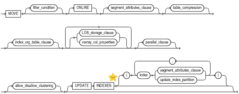
18c create sequence parameters

create sequence syntax diagram 18c

syntax diagram

Some basic stuff first

Here we go through the different parameters. Behind some of those are very complex concepts. If so, those concepts are explained in a later section. This basic section tackles the way how to set the parameter and the immediate effects of setting or not setting it.

INCREMENT BY vs. START WITH

START WITH says what the very first value will be. It can be negative.

INCREMENT BY says how the next value will be calculated. It can also be negative but not 0.

The syntax diagram is slightly misleading. It gives the impression as if we can only specify one during the creation. Either INCREMENT or START WITH, but not both. This is not true, we can create a sequence and specify both. The default for both is 1.


create sequence testseq increment by 10 start with 2;
select testseq.nextval from dual connect by level <= 3;

NEXTVAL
2
12
22

Other parameters like CYCLE and NOCYCLE can not be specified both at the same time. The syntax diagram is correct for those.

For the reminder of this document, we assume the increment is always 1 (unless clearly mentioned otherwise)

Note that we can not alter the START WITH value, but we can alter the INCREMENT BY.

Hint: The undocumented RESTART clause allows to set a new START WITH value. See section about “How to reset a sequence”.

MAXVALUE and MINVALUE

Typically we don’t have the need to set those two parameters, the defaults are good.

Facts

  • MAXVALUE and MINVALUE specify the highest and the lowest possible value a sequence can have. MAXVALUE must be greater than MINVALUE.
  • NOMAXVALUE (1028-1) is the highest possible value.
    NOMINVALUE -(1027 -1) is the lowest possible value.
  • The default for MAXVALUE is NOMAXVALUE.
    The default for MINVALUE is 1.
  • The MINVALUE can not exceed the value defined by START WITH. Or otherwise we get an error.
    ORA-04006: START WITH cannot be less than MINVALUE

CYCLE vs. NOCYCLE (default)

CYCLE specifies, that the sequence after it reached the MAXVALUE, will start again with the MINVALUE (not with the START WITH value). The theoretical maxvalue of a sequence is 28 digits. It is a bit less with scalable sequences.

Nowadays there is no compelling reason to use CYCLE.

I believe in the old days (1990 – Oracle 7) disc space was still a premium commodity. Therefore number columns were often limited to a low number of digits (5 or 6). Under certain specific circumstances a cycling sequence then might have been useful to prevent numeric or value errors. Those days are gone.

CACHE (default) vs. NOCACHE

Caching a sequence is a huge performance feature. The default setting is CACHE 20, which is good for most scenarios.  It means 20 sequence values are read from shared memory (SGA) instead from hard drive. And after that the dictionary will be updated one time.

See the section about caching considerations for more information about this very important parameter.

Demo:

create sequence mySeq cache 1000;
select sequence_name, cache_size, last_number
from user_sequences
where sequence_name ='MYSEQ';
SEQUENCE_NAME CACHE_SIZE LAST_NUMBER
MYSEQ         1000       1

select myseq.nextval from dual connect by level <= 3;
NEXTVAL
1
2
3

select sequence_name, cache_size, last_number
from user_sequences
where sequence_name ='MYSEQ';
SEQUENCE_NAME CACHE_SIZE LAST_NUMBER
MYSEQ         1000       1001

After this, we still have 997 cached sequence values.

The default value of cache 20 is a kind of sweet spot for OLTP purposes. Only when you have the need to create a very large number of sequence values in a short time, then consider to increase the cache. This typically happens during data load situations. Don’t forget to lower the cache value again after the data load is over.


ORDER vs. NOORDER (default)

It is a common misconception that we need to specify ORDER to get ordered values from a sequence object. The sequence object will always produce ordered values! Oracle did not implement some kind of random mechanism. Sequence.nextval will always give you the last value + the increment. Any kind of “randomness” comes from other things, like that you seem to have no control over who fetched the last value (multi user), when was that value inserted (seq.nextval call < insert time < commit time) and lost sequence caches.

The ORDER setting is only relevant in a RAC (Real Application Cluster) environment. And even there it should always be NOORDER (the default). Read the chapter about the performance considerations for an explaination.

Remember

ORDER on RAC = slow

ORDER on non-RAC = no effect

easy.


KEEP vs. NOKEEP (default)

This is a switch that most database developers will never need. It might be more relevant for Java developers.

In 12.2 a new feature called application continuity was introduced. It allows to capture and replay a certain workload on the database. It comes with the license options for RAC or Active Data Guard.

Problem is that a call to sequence.nextval would deliver a new value. This is not wanted for REPLAY purposes. Altering a sequence to KEEP would provide the same sequence value during the replay.

From the appendix of Oracles White paper about Application continuity:

Mutable Functions
Mutable functions are functions that can change their results each time that they are called. Mutable functions can cause replay to be rejected because the results visible to the client can change at replay.
Consider sequence.NEXTVAL that is often used in key values. If a primary key is built with a sequence value and this is later used in foreign keys or other binds, the same function result must be returned at replay.
Application Continuity provides mutable value replacement at replay for Oracle function calls if GRANT KEEP or ALTER.. KEEP has been configured.
If the call uses database functions that support retaining original mutable
values, including sequence.NEXTVAL, SYSDATE, SYSTIMESTAMP, and SYS_GUID, then, the original values returned from the function execution can be saved and reapplied at replay. If an application decides not to grant mutable support and different results are returned to the client at replay, replay for these requests is rejected.

Important to remember is that the KEEP parameter during creation has nothing to do with keeping the sequence pinned in the SGA. An example how to do that is in the “discussion about gapless IDs” section.

SCALE vs. NOSCALE (default)

SCALE is a very interesting new setting. It allows to improve the clustering factor of the index on the ID column. More details about that in the performance section.

Useing SCALE adds the session ID (SID) to the beginning of the sequence value.

SCALE has two options EXTEND and NOEXTEND (default). See how it works and differs.


create sequence myseq;

Sequence MYSEQ created.

                               NEXTVAL
--------------------------------------
                                     1
alter sequence mySeq scale;
                               NEXTVAL
--------------------------------------
          1017670000000000000000000002

alter sequence mySeq scale extend;
                               NEXTVAL
--------------------------------------
    1017670000000000000000000000000003

For sake of brevity I removed the “sequence altered.” results and “select mySeq.nextval from dual;” calls.

My session ID in this demo was 767. The 101 is the instance ID (1) + 100. So in a RAC environment, this will ensure that the values provided by different nodes will not clash. On non-RAC systems this leading part should always be 101.

NOSCALE gives us a normal sequence value of 1.
SCALE NOEXTEND gives us a sequence value of 28 digits (MAXVALUE) with a 2 at the end (last value+increment by) and a 101767 at the beginning.
SCALE EXTEND gives us a sequence value of  28+6 digits with a 3 at the end (last value+increment by) and a 101767 at the beginning.

So EXTEND adds the additional digits on top of the MAXVALUE setting, whereas NOEXTEND adds it inside the range defined by MAXVALUE.

In most circumstances – if we consider scalable sequences – we should use SCALE NOEXTEND. Just to be sure, that the generated value still does fit into the table column. For very large tables if there are already some extremly high values, we might need to use EXTEND, but I expect this situation to be very rare.

When is this useful? Only for cases when extrem performance matters. So for large or very large tables, with a lot of inserts from multiple sessions (parallel inserts).

SESSION vs. GLOBAL (default)

Sequence values do not depend on a user session. Every call to sequence.nextval will give the next incremented value regardless of which session executed this. This feature ensures that nobody gets a duplicate key.

User/Session A calls mySeq.nextval 3 times and gets 1,2,3.
User/Session B calls mySeq.nextval 3 times and gets 4,5,6.
If both sessions fetch the values almost simultaniously then A might get 1,3,4 and B might get 2,5,6. Notice that there might be gap from the perspective of a single session, but the values are still ordered for each session.

With SESSION sequences this behaviour changes. Session A calls mySeq.nextval three times and gets 1,2,3. Session B calls mySeq.nextval three times and also gets 1,2,3. The values are not shared between sessions.

Where do we need this? Only for global temporary tables (GTT). The data in a GTT  persists for the duration of a session (alternatively until commit) and then is gone. Same behaviour for the SESSION sequence – the generated sequence values only persist for the duration of the session.


Practical considerations

For most cases the default settings are perfect.

Only if you encounter issues (performance  or unusual number of gaps) or if your data has some special scenarios (batch ETL jobs, very large number of rows) then you should start thinking about tinkering with the default settings.

The following sub chapters discuss common questions and show cases how to work with sequences to solve some typical tasks.

How to avoid reusing the same ID in different dbs

Sometimes we have a distributed database. Especially for global companies each region might have its own database. The data for the different regions still needs to be comparable. And sometimes the data will be consolidated or exchanged. In such cases it helps, if the ID values do not overlap.

One way to do that is to use the INCREMENT parameter. On database 1 we use a sequence object starting by 1 and and increment of 10. So this will give IDs like 1, 11, 21, 31, 41,….

create sequence testseq increment by 10 start with 1;

On Database 2 we use a sequence starting with 2 and increment 10. This will work up to 10 regions. So this will give IDs like 2, 12, 22, 32, 42, ….

create sequence testseq increment by 10 start with 2;

Result is that those values do not overlap. There are other (and possibly better) ways to solve the situation, like sys_guid(). But this is a fairly easy and stable concept.

Caching considerations

If the sequence is used very infrequently, then you can set it to NOCACHE. For example if you have an staff table; I don’t expect that new personell is hired every second. Typically it will be a few people per month (depends on the size of your company of cause). For such low frequency inserts performance doesn’t matter. You can set the sequence object to NOCACHE or to a very low cache value. However if you do a large data import, consider to increase the cache size before running that data load.

Does setting a larger cache size need more SGA memory?

No.

Or to explain it with Tom Kytes words

All we need to keep in the cache is:

the sequence on disk was N
the cache size is M
the current value is X

As long as X is less than N+M – we just increment X when someone calls NEXTVAL.

we do not need to keep in the cache “N, N+1, N+2, … N+M-1”, we just keep N, M and X and increment X when someone asks for a new sequence value. When X=M, we update SEQ$ and reset N in the cache.

So, cache 1000 and cache 20 take the same amount of space in the cache.

How to reset a sequence?

There are three general ways to set a sequence to a different value.

  1. Call sequence.NEXTVAL so often until you reach the target value
  2. Manipulate the increment parameter using a negative increment. Call nextval once. Reset.
  3. Restart the sequence (new undocumented feature)

The first way usually is not practical. A noticable exception might be, if you manually added some data without using the sequence and you want to jump over those few values.

If you want way 1, then the CONNECT BY LEVEL clause helps to do it quickly.


select myseq.nextval from dual connect by level <= 996;


And here is a demo for way 2:
Preparation setup


drop sequence mySeq;
create sequence mySeq cache 1000;
set autotrace traceonly statistics
select myseq.nextval from dual connect by level <= 996;
set autotrace off
select myseq.nextval from dual;
   NEXTVAL
----------
       997

The “set autotrace traceonly” command works in sql*plus. I used it here to avoid printing 996 values onto the screen. It is not relevant for the demo itself.

The current value now is 997 but we want that the next call to nextval should give us 1.

Now reset the sequence.

alter sequence mySeq increment by -996 nocache;
select myseq.nextval from dual;
alter sequence mySeq increment by 1 cache 1000;

After this code, the very first session that calls myseq.nextval, will see 2 as the value returned.

If we really need to see 1 we also must lower the MINVALUE. Because INCREMENT BY can not result in anything lower than the MINVALUE (ORA-08004: sequence MYSEQ.NEXTVAL goes below MINVALUE and cannot be instantiated).

alter sequence mySeq increment by -997 nocache minvalue 0;
select myseq.nextval from dual;
alter sequence mySeq increment by 1 cache 1000;
select myseq.nextval from dual; 

Notice that we incremented now by -997 instead of -996 and that we are calling nextval twice. We can not reset the minvalue to 1 during the second ALTER sequence command, because that also would violate the rules (ORA-04007: MINVALUE cannot be made to exceed the current value). Easyiest solution is to let it stay at 0.

Using NOCACHE is important, to avoid having issues with the stored last_value. Also check the increment by and the cache setting, before you alter the sequence. If the increment by is different, then you need to change the above code and probably need to call nextval a second time.

In 18c we got a third option to reset a sequence – the RESTART option.


ALTER SEQUENCE mySeq RESTART;

This is currently undocumented.

Thanks to Roger Troller for makeing me aware about it (Blog).

I tested it a little bit further and found out two more things.

  • We can already use it in 12.2.0.1. Which makes sense, since 18c is really just 12.2.0.2.
  • And we can combine it with the START WITH clause.

So the following works !

alter sequence testseq_20 restart;
VAL1
1
alter sequence testseq_20 restart start with 15;
Sequence TESTSEQ_20 altered.
select testseq_20.nextval val1 from dual;
VAL1
15

Very convinient. This should be the preferred way to reset a sequence whenever you need to do that.

Not recommended is to drop and recreate the sequence. While this will also allow us to set a new START_WITH value, it has a major drawback. All references to the seqeunce are then broken. Especially all privileges are lost, like GRANT SELECT on #sequence to #schema.


Can we use an ID from a sequence to order by insert time?

Short answer no. The order of inserts and the order of sequenced values often match but are not guaranteed to match.

Detailed answer: Usually it works.

I very often use a ID column filled by a sequence as a second order criteria. For example I typically sort a logging table – where trace information is written – by the insert date and the LOG_ID (sequence based PK ).

order by insert_date desc, log_id desc

The insert date (if it is a date) is only accurate to the second. Even if it is a timestamp there might have been multiple inserts at the same fraction of a second. The log_id is a perfect second order criterium.

We can safely assume, that the inserts that were done from the same session, have ordered sequence values. There might be gaps, but the sequence values will be produced in the same order as we did the inserts. There can be ID values in between, that are from a different sessions. But for trace log information, usually it does not matter if a different session is ordered before or after our session. However the data from one session should be correctly ordered. And this is guaranteed.

Is cycling useful?

I never had the need of cycling sequences. I firmly believe if you think you need those, you have a much deeper problem somewhere else. It would probably better to solve that problem, instead of useing a cycling sequence.

With 18c we get SESSION sequences. For some cases where CYCLE was considered in the past, a SESSION sequence might be the better choice.

Also ROWNUM and the analytic function ROW_NUMBER can be used to create consecutive values at time of select, instead of a sequence providing those values at time of insert.

Discussion of gapless IDs

This is a problem/question I often encountered: How to make a sequence gapless?

TL;DR: You don’t need to. The effort and the restrictions to make an ID column gapless is to high in (almost) all use cases.

The sequence object can and does provide gapless numbers. In a multi user environment we just can not reliably use the provided values to store them in a gapless way. Even in a single user environment, the stored IDs could be deleted. So one consequence of the gaplessness requirement, would be to forbid delete operations.

The main point is that almost all the things that will create “holes” in an ID column are under our control. It is not the Oracle database that can not provide gapless sequences. It is the complexity of the business rules combined with performance requirements in a multi user environment, that make it almost impossible to have an ID column without potential gaps.

Performance + Multi User + Gapless IDs build a triangle of goals that exclude each other. We can not reach all three goals at the same time, one needs to suffer. However those goals do not react in the same way, when we sacrifice one a tiny bit. So let’s investigate what happens then:

We still can not reach good performance (instead of very high performance) if we need multi user capability and gaplessness at the same time. To enable this we need to serialize access to the whole table. Which in turn means only one session can write into the table and all other sessions will need to wait until the other session finishes the whole transaction.

We can have very high performance and gaplessness if we only have a single user. But as soon as a second user wants to write at the same time, we need to introduce severe serialization of the whole transaction, just to ensure gaplessness. And this means performance drops immensely. Btw. this is how MS Access works. Only one user can write into the so-called database.

But we can get almost gapless IDs and still have very high performance for multiple users. Almost gapless means, we sometimes might have gaps in our sequence, but this situation is rare. This is the default behaviour of Oracle sequences.

How do we get gaps in our IDs?

a) a record in our table was deleted.
b) the insert run into an error
(remember sequence.nextval is called a tiny moment before the insert is executed).
c) Somebody called sequence.nextval but didn’t use the value.
d) The sequence cache was lost. One way how this happens is if the database decides that other objects need to be in SGA memory and the sequence wasn’t called for a longer time.

By pinning the sequence we can avoid situations where the sequence cache ages out of the shared pool. A better alternative is to size the shared pool appropriately, so that in general sequence caches will not age out of it.

execute sys.dbms_shared_pool.keep(owner.mySequence,'Q');

This still doesn’t guarantee gapless IDs, but for most use cases it would be good enough.

The oracle docs about skipping cached numbers:

18.1 Database Admin Guide – Managing Sequences
The database might skip sequence numbers if you choose to cache a set of sequence numbers. For example, when an instance abnormally shuts down (for example, when an instance failure occurs or a SHUTDOWN ABORT statement is issued), sequence numbers that have been cached but not used are lost. Also, sequence numbers that have been used but not saved are lost as well. The database might also skip cached sequence numbers after an export and import. See Oracle Database Utilities for details.

A normal or immediate shutdown of the database will not loose sequence numbers. Instead the database will update the data dictionary (table sys.seq$) with the last used value.  Unfortunatly most DBAs prefer to shutdown a database using abort, since they don’t bother enough about user sessions.

Sequence Performance

Why is a sequence fast and how can we use it in the most performant way?

Oracle invented sequences with performance in mind. They provide a way to create surrogate keys in a multi user environment while minimizing serialization.

Basic working of an Oracle sequence

A sequence is just an entry in the dictionary table sys.seq$.

desc sys.seq$;

Name       Null?    Type 
---------- -------- ------------ 
OBJ#       NOT NULL NUMBER 
INCREMENT$ NOT NULL NUMBER 
MINVALUE            NUMBER 
MAXVALUE            NUMBER 
CYCLE#     NOT NULL NUMBER 
ORDER$     NOT NULL NUMBER 
CACHE      NOT NULL NUMBER 
HIGHWATER  NOT NULL NUMBER 
AUDIT$     NOT NULL VARCHAR2(38) 
FLAGS               NUMBER 
PARTCOUNT           NUMBER

The highwater column is the same as the last_number column in the view user_sequences.

When a sequence fetches a new sequence value (using .nextval) then the dictionary table needs to be read and the row needs to be updated with the new value. Now if multiple sessions do that, then one would have to wait for the other. This is called serialization. To avoid that issue, Oracle uses two clever mechanisms.

  1.  The dictionary table is updated using an autonomous transaction. So the value is stored and other sessions can see it, even if the main transaction (from the user session) is not finished.
  2. The new highwater value that is stored, is not the next value, but it is the value + the cache. Any call to sequence.nextval will first read from the sequence cache and only once the numbers there are exhausted, it will read from the table and update it.

It is of cause possible to write a similar mechanism ourselfs with our own table. And I have seen projects where they did exactly that. But it is very hard to do properly and even then will not beat the performance of the original sequence.  So you would need a very special business case to justify writing your own sequence mechanism.

Speed it up

If you aim for maximum performance there are some considerations to do.

  1. You must use a sequence cache. The cache size also plays an important role. For most OLTP tables the default setting of cache=20 is a very good choice. However when you do large dataloads, then a much larger cache size is advisable. There is a diminishing returns effect. Doubleing the cache does not double the performance.
  2. On a RAC you really should use NOORDER. The ORDER keyword is only relevant for real application clusters. Using ORDER would try to synchronize the sequence caches over all cluster nodes. This is extremly bad for the performance. Useing NOORDER gives each RAC node a separate sequence cache. Which also means that an insert on node1 might have sequence value 1 and the next insert on node2 might have a sequence value 1001. The third insert on node1 again would use value 2.
  3. Sequences should be used as late as possible. There is usually no need to fetch a sequence value first and then do the insert later. Use the sequence while doing the insert. Either by adding it to the insert statement, or via a database trigger or since 12c as an identity column or a default on NULL column setting. Using the 12c mechanics allows to avoid the database trigger. This results in much better performance, as I have shown in a previous blog post.
  4. Consider scalable sequences for large tables if you are on 18c already. The effect can not be seen immediatly, but scalable sequences should give a better and more stable performance in the long run.
    For small and medium sized tables I expect scalable sequences to be slower than non-scalable sequences (because a bigger number needs to be stored). I didn’t test the effect, but a normal (small) sequence value only needs 2-6 bytes, wheras a scaled sequence value needs always 15 (NOEXTEND) or 18 (EXTEND) bytes. These bytes are used by the table column, the unique index that supports the primary key (PK), all foreign key (FK) columns pointing to the PK and the indexes supporting those FKs.


If you need the value of the sequence later in your code again you can either use .currval (not recommended) or use the returning clause to give you the generated ID.

best practice: returning clause

Several SQL and PL/SQL DML commands have a returning clause. It allows to get back data that is created or manipulated while the DML (insert or update) is running.

The most common usage is to return the ID value, that is filled by a database trigger (or an identity column) so that this ID can now be used furthermore in the same session or transaction or to be returned back to the client. For example to insert any child records or to show the freshly generated record in a GUI report.


insert into super_emp (first_name, last_name, hire_date)
values ('Bruce', 'Banor', trunc(sysdate))
returning id into :ID;

print :ID;

ID
--------------------------------------------------------------------------------
9

The returning clause is more typical in pl/sql. Here is an example using a record of %rowtype. We can even return the generated ID value directly into the record.

declare
r_super_emp super_emp%rowtype;
begin
r_super_emp.first_name := 'Hal';
r_super_emp.last_name := 'Jordan';
r_super_emp.hire_date := trunc(sysdate);

insert into super_emp
values r_super_emp
returning id into r_super_emp.id;

sys.dbms_output.put_line('New ID = '||r_super_emp.id);
end;
/
New ID = 10


Identity columns

Identity columns and Default on null are a great enhancements in db version 12.1.

It allows us to use a sequence as late as possible (while inserting). But without the need for a before row insert table trigger. This improves insert performance dramatically. A trigger is plsql based. It runs during the execution of a SQL DML statement (insert). Because of that a context switch from the SQL to the PL/SQL engine (and back) is needed. If we can avoid the trigger completly we can avoid the context switch and this will improve performance considerably.

I made some tests and under very favourible circumstances (nothing else inserted but the ID) the insert performance was 900% faster using IDENTITY or DEFAULT columns instead of a trigger.

With DEFAULT ON NULL we would still create the sequence by ourself. Which also means we know the name. With IDENTITY the sequence is automatically created and maintained by Oracle.

The name of the generated sequence will always begin with “ISEQ$$_”.

demo


create table test
( id number generated by default on null as identity (start with 20) primary key
);

select table_name, column_name, identity_column, default_on_null, data_default
from user_tab_columns;

TABLE_NAME COLUMN_NAME IDENTITY_COLUMN DEFAULT_ON_NULL DATA_DEFAULT
TEST ID YES YES “SCHEMANAME”.”ISEQ$$_10707661″.nextval


Drawbacks

It can be problematic to use identity columns over a database link. Especially if the ID value is needed. The main issue is that the returning clause does not work over a db link and there are no good alternatives for identity columns. This works slightly better with “default on null”. We know the sequence object and can use it to fetch the id value over a DB link first and use it then later for the insert. Not performant at all, but it works.

We also can not directly alter an existing ID column into an IDENTITY column. Although it is possible to modify an existing identity column (for example switching between generated always and generated by default on null).

Another minor inconvinience is that the system generated sequence will still be there when the table is dropped. At least as long as the table is still in the recycle bin.

There were also some other very special bugs using identity columns. All have workarounds, but my experience is, that default on null is slightly less error prone.


Index contention and Scalable Sequences

Scalable sequences where secretly introduced in 12.1.0.1 but only documented in 18.1.

Richard Foote did a three part series about scalable sequences that covers all you need to know.

The basic problem has to do with index contention.

To give a very brief explanation: when we have an ID column that is inserted using a sequence the index -over time- will become unbalanced. Because new values will only be added to the right side of the index leaf block splits will happen there frequently. Sometimes it will be 50-50 block split and the space in those blocks usually will not be filled up.  This eventually leads to a heavily right (un)balanced index tree.

Such a block split is a very ressource intensive operation and other sessions will need to wait for it. If you see a high number of “enq: TX – index contention issue” wait events (check MOS 873243.1) the reason could be those index block splits.

One workaround for the index contention problem in the past was to use a REVERSE KEY index. But this created other performance problems, like the CBO will not do any range scans on that index.

Scalable sequences are a slightly better solution to avoid those index contention issues (hot index blocks). Because they have the session ID in front of the number, values provided by a scalable sequences are distributed more evenly over the index. At least as long as multiple sessions do the insert.


Export and Import

consistency issues

When you do an export of a database or a schema it is crucial to do a time consistent export using

exp ... consistent=Y ...

Why? Otherwise the sequence object including the current value as start with is exported first. And later the tables with their data. Which means, that in between some session could call sequence.nextval and use up a value. You won’t notice the issue during import. But as soon as an insert in the imported schema happens, you will get an dup_val_on_index error, because the table has an ID value already, that the sequence generator just provided.

sys warning

Consistent=Y does not work as SYS. So never export data as SYS! The reason is that sys can not do read only transactions. Using SYSTEM is fine.

datapump

For datapump the equivalent to consistent=Y is the flashback parameter.

expdp ... flashback_time=systimestamp ...

There is also a flashback_scn parameter. Both do a time consistent export.

And since 11.2 there is a legacy mode for datapump, which allows to use consistent=Y (it is rewritten into the flashback_time parameter).


Other ways to generate ordered numbers

Sometimes a sequence is not the best way to generate ordered numbers. For example when we want to sort entries from a detail table based upon their parent keys. Each detail record should start with 1 for each parent entry. A sequence is not the proper tool to get such values.

Alternatives are ROWNUM, the analytical function ROW_NUMBER() and certain ways to create lists in SQL, for example by using hierachical queries with CONNECT BY.


Further reads


plsql collection lookup with multiple keys

problem scenario

A recent question on otn asked how to access a plsql collection using multiple keys.

It is a typical scenario to build a second collection, to be able to access the main data in the first collection. The second collection fulfills the same role as an index on a table. It allows fast access to the main data record. I usually call the second collection an “index collection”.

Here is an article by Steven Feuerstein who explains the concept of index collections in more detail: https://blogs.oracle.com/oraclemagazine/on-the-pga-and-indexing-collections

But the forum question was not how to do a simple key => value lookup, but instead have two keys (based upon record set values) and use them to access the main collection.

solution

There are two general ways.
Combine the keys into a single key or build a nested collection. I will show a quick example for both ways.

Way 1) Combined key

We can consolidate the two keys into one single key. Typically using some delimiter. And then use that combined key for the index_collection.

combinedKey := key1||':'||key2;

Of cause we need to make sure the delimiter is some value that does not exist in any of the keys.

Example
If you try to copy and run this example please note that the syntax highlighter removed the label “build_index”
You might want to add this again, just after the “– index data” comment.

set serveroutput on
declare
  cursor c is (select trunc((level+2)/3) lvkey, chr(ASCII('A')+mod(level*2,3)) letter, round(dbms_random.value(1,100)) val 
               from dual 
               connect by level <=10
                );
  type tabdata_t is table of c%rowtype index by binary_integer;   
  tabdata tabdata_t;
  
  type keylookup_t is table of binary_integer index by varchar2(100);
  keylookup keylookup_t;
begin
  -- load data
  open c;
  fetch c 
  bulk collect into tabdata; -- notice no limit clause here. For larger record sets you need to use a loop and LIMIT!
  close c;
  
  -- index data
  <>
  for i in 1..tabdata.count loop
    keylookup(to_char(tabdata(i).lvKey)||':'||tabdata(i).letter) := i;
  end loop build_index;
  -- index is now complete. 
 
   -- Test the index first
  dbms_output.put_line('Index 1B=>'|| to_char(keylookup('1:B')));
  dbms_output.put_line('Index 3A=>'|| to_char(keylookup('3:A')));

  -- now fetch the data using the index
  dbms_output.put_line('Data 1B=>'|| tabdata(keylookup('1:B')).val);
  dbms_output.put_line('Data 3A=>'|| tabdata(keylookup('3:A')).val);
end;
/

Output

Index 1B=>2
Index 3A=>9
Data 1B=>32
Data 3A=>67

PL/SQL procedure successfully completed.

Way 2) collection of collection

A collection can be part of another collection. Nesting collections means we could do a lookup using two (or more) key values where each key is used for one collection.

lookup(key1) => col2
this returns a collection (e.g. col2). We can access the elements of the collection using the second key.

col2(key2) => element

or the short form:
lookup(key1)(key2) => element

For readability we could add a record layer in between, but that is not neccessary.
lookup(key1).list(key2) => element

Example
Notice the definition of the index collection is in line 14 with the matching type definitions in line 11 and 12.

set serveroutput on
declare
  cursor c is (select trunc((level+2)/3) lvkey, chr(ASCII('A')+mod(level*2,3)) letter, round(dbms_random.value(1,100)) val 
               from dual 
               connect by level <=10
                );
  type tabdata_t is table of c%rowtype index by binary_integer;   
  
  tabdata tabdata_t;
  
  type letterlookup_t is table of binary_integer index by varchar2(10);
  type keylookup_t is table of letterlookup_t index by binary_integer; -- number not allowed!
  
  keylookup keylookup_t;
  empty_key letterlookup_t;
begin
  -- load data
  open c;
  fetch c 
  bulk collect into tabdata; -- notice no limit clause here. For larger record sets you need to use a loop and LIMIT!
  close c;
  
  -- index data
  <>
  for i in 1..tabdata.count loop
    if keylookup.exists(tabdata(i).lvKey) then
      if keylookup(tabdata(i).lvKey).exists(tabdata(i).letter) then 
        -- same key twice?
        -- maybe add the values, maybe raise an error
        raise dup_val_on_index;
      else  
        dbms_output.put_line('build index KEY='||tabdata(i).lvKey||',+letter='||tabdata(i).letter);
        keylookup(tabdata(i).lvKey)(tabdata(i).letter) := i;
      end if;      
    else -- key not in index yet
      dbms_output.put_line('build index +KEY='||tabdata(i).lvKey||',+letter='||tabdata(i).letter);
      keylookup(tabdata(i).lvKey) := empty_key;
      keylookup(tabdata(i).lvKey)(tabdata(i).letter) := i;
    end if;      
      
  end loop build_index;
  -- index is now complete. 
 
  -- Lets access the data using some combinations of keyLv and letters
  -- Test the index first
  dbms_output.put_line('Index 1B=>'|| to_char(keylookup(1)('B')));
  dbms_output.put_line('Index 3A=>'|| to_char(keylookup(3)('A')));
  --dbms_output.put_line('1F='|| keylookup(1)('F')); -- this will raise NO_DATA_FOUND
  
  -- now fetch the data using the index
  dbms_output.put_line('Data 1B=>'|| tabdata(keylookup(1)('B')).val);
  dbms_output.put_line('Data 3A=>'|| tabdata(keylookup(3)('A')).val);
  
end;
/

Output
build index +KEY=1,+letter=C
build index KEY=1,+letter=B
build index KEY=1,+letter=A
build index +KEY=2,+letter=C
build index KEY=2,+letter=B
build index KEY=2,+letter=A
build index +KEY=3,+letter=C
build index KEY=3,+letter=B
build index KEY=3,+letter=A
build index +KEY=4,+letter=C
Index 1B=>2
Index 3A=>9
Data 1B=>62
Data 3A=>34

PL/SQL procedure successfully completed.

If we try to access a collection that does not exist we get an error (usually no_data_found). Since the index collections are always sparse, this is something to keep in mind. If you are not sure if the key combination is already indexed, then either check for existence or react on the NO_DATA_FOUND.

comparison

It is not easy to compare the two approaches. The first way looks slightly less complex. It depends also how familar other developers are with collections and especially with nested collections. For many the double parenthesis syntax “myCol()()” is a little complicated at the beginning.

For very complex scenarios the first way might be the better way. It depends on data distribution (the more sparsly populated the key combinations are, the better is this way) and on how many keys (=dimensions) we have.

I once measured the performance in a system where we needed 5 dimensions (5 different keys) to access some data. The combined key lookup was faster than building a complex collection of collection of collection of collection. But the additional time to concat the key values in the end also was a large performance burden.

So in my specific case
lookup('A:B:C:D:E') >>> lookup('A')('B')('C')('D')('E')

I do not think this performance experience is representativ.

conclusion

It is possible to use two keys as an index collection to lookup data in the main collection. Nested collections is a tool that every plsql developer should know about. Only when we know our tools, we can decide when to use them or when not.

Tackling “cursor: pin S wait on X” wait event issue

Problem description

I found the following interesting issue by accident during an performance analysis using ASH and real time SQL monitoring.

We (@gassenmj and myself) saw that all connections from an application server connection pool were suddenly “hanging” at the same SQL statement. The single session did have wait times ranging from a few seconds up to 30 seconds and more. Additionally some CPU throttleling was going on.

After a couple of minutes the system healed itself and went back to normal behaviour. Those were the symptoms. Although that was not directly related to the performance analysis we had planned, we decided to investigate further.


Problem indicators

Here follows a list of statements that helped to analyze the problem.

check session infos

select * from v$session;

select * from v$session_wait 
--where sid=sys_context('userenv','sid')
order by wait_time+seconds_in_wait desc;

We saw a high number of “cursor: pin S wait on X” events with a high wait time. At that time I didn’t know what the issue was, but it was obvious that there is some kind of problem. If you encounter a high number of sessions all with the same wait event, then you might want to investigate further. Especially if the system seems generally slow while this event happens.

check the active session history (ASH) report

Please note that accessing the ASH report requires an enterprise edition and a licensed diagnostics pack. Do not try to run any select against v$active_session_history in a standard edition!

If you are allowed to use ASH, then run the following selects for a quick check. ASH typically holds information only for the last 30 minutes. Then the data is consolidated into the AWR report. If possible I prefere ASH because it samples information every second.

-- ash info
select ash.sample_time, ash.session_id, ash.session_serial#, ash.sql_id,  
       ash.event, -- ash.p1, ash.p1text, ash.p2, ash.p2text, ash.p3, ash.p3text,
       ash.wait_time, ash.time_waited, 
       ash.blocking_session, ash.blocking_session_serial#,
       ash.in_parse --, ash.in_hard_parse, ash.in_sql_execution
from v$active_session_history ash
where ash.event = 'cursor: pin S wait on X'
order by ash.sql_id, ash.sample_time;

Eventually the data is moved into the dba_hist_active_sess_history view.

-- awr info
select sql_id, sample_time, session_id, wait_time, time_waited, module, machine
from dba_hist_active_sess_history
where event = 'cursor: pin S wait on X'
order by sql_id, sample_time;

We can consolidate the infomation over all sessions that seem to be connected to the issue. This summary statment also includes the session that seems to cause the issue.

-- ash summary
with sum_by_session as (
        select ash.sql_id, ash.session_id, 
               trunc(ash.sample_time,'HH') timeframe, min(ash.sample_time) min_time, max(ash.sample_time) max_time,
               sum(ash.wait_time) + sum(ash.time_waited)  total_wait,
               ash.event, ash.p1, ash.p1text, ash.p2, ash.p2text, ash.p3, ash.p3text, ash.in_hard_parse
        from v$active_session_history ash
        join v$active_session_history sqlids on sqlids.sql_id = ash.sql_id
        where (ash.event like 'cursor: pin S%' or ash.in_hard_parse = 'Y' )
        and sqlids.event = 'cursor: pin S wait on X'
        group by  ash.sql_id,  ash.session_id, ash.event, ash.p1, ash.p1text, ash.p2, ash.p2text, ash.p3, ash.p3text, ash.in_hard_parse
                 ,trunc(ash.sample_time,'HH')
         )        
select s.sql_id, to_char(s.timeframe,'dd-Mon-RR HH24') timeframe,
       to_char(min(s.min_time),'HH24:MI:SS')||'-'||to_char(max(s.max_time),'HH24:MI:SS') timeperiod, 
       round(sum(total_wait)/1000000,2)  total_wait_in_s,
       s.event, s.p1, s.p1text, s.p2, s.p2text, s.p3, s.p3text, s.in_hard_parse, 
       listagg(s.session_id,',') within group (order by s.session_id) as sids
from sum_by_session s              
group by s.sql_id,  s.event, s.p1, s.p1text, s.p2, s.p2text, s.p3, s.p3text, s.in_hard_parse, s.timeframe
order by s.sql_id, s.in_hard_parse desc, s.timeframe;

Here is some sample output from a test database. It shows a list of sessions (column SQLIDs) that are waiting for cursor: pin S wait on X.

SQL_ID	   TIMEFRAME	    TIMEPERIOD	   TOTAL_WAIT_IN_S 	EVENT			P1		P1TEXT	P2		P2TEXT	P3		P3TEXT	IN_HARD_PARSE	SIDS
a7s0bjm8467xg	22-mai-18 04	04:21:10-04:21:10	0,46	cursor: pin S wait on X	3494059951	idn	674309865472	value	21474836480	where	N	20,255,301
cq42gcnqfs5vd	22-mai-18 04	04:21:09-04:21:09	0,04				1		file#	31620		block#	1		blocks	Y	247
cq42gcnqfs5vd	22-mai-18 04	04:21:10-04:21:10	0,03				1		file#	31323		block#	1		blocks	Y	247
cq42gcnqfs5vd	22-mai-18 04	04:21:09-04:21:10	610,9	cursor: pin S wait on X	753669997	idn	1060856922112	value	21474836480	where	N	18,51,70,73,127,169,191,229,326,379,390,426,436,456
3320xrzqy5t5c	22-mai-18 12	12:21:13-12:21:13	0				1		file#	22750		block#	1		blocks	Y	269
3320xrzqy5t5c	22-mai-18 12	12:21:13-12:21:13	0,11	cursor: pin S wait on X	3991069868	idn	1155346202624	value	21474836480	where	N	314
76fxznczqskp8	22-mai-18 00	00:21:07-00:21:07	0				1		file#	589		block#	1		blocks	Y	15
76fxznczqskp8	22-mai-18 00	00:21:08-00:21:08	0,05				1		file#	31323		block#	1		blocks	Y	15
76fxznczqskp8	22-mai-18 04	04:21:08-04:21:08	0,04				1		file#	507		block#	1		blocks	Y	73
76fxznczqskp8	22-mai-18 00	00:21:07-00:21:08	404,66	cursor: pin S wait on X	1064061608	idn	64424509440	value	21474836480	where	N	8,67,90,151,167,193,221,253,314,351,364,367,419,456
76fxznczqskp8	22-mai-18 04	04:21:08-04:21:08	419,54	cursor: pin S wait on X	1064061608	idn	313532612608	value	21474836480	where	N	18,51,70,127,169,191,247,326,379,390,426,436,456

In this example we had many sessions with the “cursor: pin S wait on X” wait event for the cursor “cq42gcnqfs5vd”. Those sessions combined waited for more than 10 minutes! And we also see two lines for the session that created this cursor (hard_parse=Y). Two lines because the hard parse took considerable time and ASH samples every second. The P2 info changed during that (last two bytes changed). I assume this means that the hard parse was progressing.

In general the summary statement shows if this wait event happend recently and also that many sessions where waiting for this event.

Finding the problem statement

We can use v$sql or v$sqlarea.

select * --sql_id, sql_text, sql_fulltext 
from v$sql 
where sql_id = 'cq42gcnqfs5vd';

or

select sql_id, module,
       sql_fulltext,
       cpu_time, elapsed_time, concurrency_wait_time, 
       version_count, parse_calls, invalidations
from v$sqlarea
where sql_id = 'cq42gcnqfs5vd';

The column SQL_FULLTEXT will hold the statement. But this information might age out of the SGA. So the sooner after the issue you run this the better. The good news is that the hashed sql_id is stable. Meaning if the same statement is run later again, you will see the same sql_id. And since we are investigating an issue that happened because the exactly same statement was run several times at the same moment (many sessions where waiting), there is a good chance that we get lucky and see this command in v$sql.

historical comparison

Very useful are the event_histograms. It can give an indication how severe the problem is. If we see a recent LAST_UPDATE_TIME for one of the high numbers (>= 4096) then some action might be needed. Also the v$event_histogram view helps to monitor if the issue disappears or is lowered once it is resolved.

select * from v$event_histogram 
where event = 'cursor: pin S wait on X';
EVENT#	EVENT			WAIT_TIME_MILLI	WAIT_COUNT	LAST_UPDATE_TIME
282	cursor: pin S wait on X	1		393	22.05.18 07:09:40,837552 +02:00
282	cursor: pin S wait on X	2		72	06.05.18 20:21:14,069132 +02:00
282	cursor: pin S wait on X	4		302	19.05.18 20:52:37,773557 +02:00
282	cursor: pin S wait on X	8		2043	22.05.18 07:09:41,041724 +02:00
282	cursor: pin S wait on X	16		6586	22.05.18 01:07:19,804808 +02:00
282	cursor: pin S wait on X	32		14719	22.05.18 07:09:41,054201 +02:00
282	cursor: pin S wait on X	64		16058	22.05.18 12:21:14,725227 +02:00
282	cursor: pin S wait on X	128		7514	22.05.18 12:21:13,702598 +02:00
282	cursor: pin S wait on X	256		10496	22.05.18 07:09:40,366636 +02:00
282	cursor: pin S wait on X	512		11360	22.05.18 07:09:40,364821 +02:00
282	cursor: pin S wait on X	1024		2123	22.05.18 07:00:05,691792 +02:00
282	cursor: pin S wait on X	2048		2240	22.05.18 04:21:11,172316 +02:00
282	cursor: pin S wait on X	4096		284	03.05.18 12:22:09,853604 +02:00
282	cursor: pin S wait on X	8192		169	30.04.18 16:22:30,975458 +02:00
282	cursor: pin S wait on X	16384		180	30.04.18 16:22:30,985937 +02:00
282	cursor: pin S wait on X	32768		31	19.09.17 18:50:00,401702 +02:00
282	cursor: pin S wait on X	65536		2	04.05.16 22:09:14,572347 +02:00

I run this on May 22nd. We see mutex sleeps for up to 2 seconds (column wait_time_milli = 2048) at 4 a.m. And a high number of mutex sleeps for 1 second at around 7 a.m. Nothing too critical but so that it might be worth checking what is going on. More about mutex sleeps in the section that explains the problem.

We also see an entry for 16 seconds from 30th of April. This was the time before we fixed the problem. The event history shows that since that time, we never had such long sleeps anymore. Which proves that our fix is working.

What the event histogram does not show, is that the waits from May 22nd and from April 30th are from a different sql_ids. So it give us only a very crude monitoring.

Event detail and mutex analysis

select * 
from GV$MUTEX_SLEEP_HISTORY
where blocking_session = 247;

This should show several sesssions during the problematic time frame. The location is the most interesting column. It will probably be this location

kkslce [KKSCHLPIN2]

We can use this location to check out the general mutex sleep history.

select MUTEX_TYPE,LOCATION,REQUESTING_SESSION,BLOCKING_SESSION,SLEEP_TIMESTAMP
from GV$MUTEX_SLEEP_HISTORY
where location='kkslce [KKSCHLPIN2]'

And to get an impression about the severity of the issue, lets compare the event against other mutex sleeps.

select * from v$mutex_sleep
--where location='kkslce [KKSCHLPIN2]'
order by sleep time desc;

Example result

MUTEX_TYPE	LOCATION	SLEEPS	WAIT_TIME
Cursor Pin	kkslce [KKSCHLPIN2]	1555183	0
Library Cache	kglpndl1  95	116623	0
Library Cache	kglpin1   4	107578	0
Library Cache	kgllkdl1  85	105747	0
Library Cache	kglhdgn2 106	83336	0
Library Cache	kglllal3 111	45584	0
Library Cache	kgllkc1   57	41674	0
Library Cache	kglpnal1  90	37040	0
Library Cache	kglget2   2	12203	0
Library Cache	kgllldl2 112	11882	0
Cursor Pin	kksfbc [KKSCHLFSP2]	11303	0
...

A high number of sleeps here shows that we have some issue.

But enough about such statements. I will explain a little why they are relevant for the problem and also what kind of problem there is.

Some technical background information

There are several recommended publications that helped me to understand and solve the issue. See links to Tanel Poder and Jonathan Lewis articles in the link section at the end of this post.

About this wait event: doc about “cursor: pin S wait on X”

The doc explains a little bit what happens. This wait event occurs when a session requires a shared mutex pin, while another session holds an exclusive mutex pin. Mutex pins are essentially locks on memory objects.

It is a lock to create the execution plan for a statement. The mutex organizes access to a shared cursor. During a hard parse the cursor (=execution plan) is created. The hard parse sets the exclusive lock. Other sessions are checking if there is already a cursor for the SQL statement (based upon the hashed sql_id). This is done by a shared pin call (cursor pin S). However the first session (247 in my case) did not free up this ressource yet, because it is still hard parsing. That is why we see a cursor: pin S wait on X for all the other sessions.

Problem cause

The issue was caused by a select that was extremly expensive to (hard) parse but which was very fast to execute.

The hard parse needed several seconds (usually 9 but up to 24 seconds). Any consecutive statement call was a soft parse using bind variables and executed in way less than 1 second.

This statement was send by some java application at the exact same time to all sessions in the connection pool. So the exact same statement, but with different bind parameters needed to run.

Each database session did this:

  • First it builds a hash (SQL_ID) for the sql statement.
  • Then it searches in the SGA if an entry for this SQL_ID already exists in a memory lookup table.
  • Since another session, at the same time, already tries to create an execution plan (hard parse). Therefore the later session waits for the outcome of this. This is a mutex wait.
  • The mutex then goes to sleep for a short time.
  • It wakes up and since the hard parse is still running, it goes to sleep again. This time a little longer.

The problem with mutex sleeps is twofold.

  • the sleep times tend to increase exponentially. We can see this in the mutex_sleep_history and event_histogram views. It starts with 1 microsecond,
    but very soon reaches an order of several seconds.
  • When a mutex tried to access a latch and sleeps on it – the latch is not free for other sessions to grab it. This can throttle the CPU.

So the mutex sleeps get longer and longer while the hard parse is still running.
Eventually the next mutex sleep will be longer than what the original hard parse time was. So even if the blocking session finished, the waiting session still doesn’t execute because the mutex sleeps now for the next 8 or 16 seconds. This can cascade to other sessions. I have seen total wait times of more than 30 seconds because of this cascading effect.

The process is partially documented (shared pool check), although not in enough detail to cover this mutex problem scenario.

For more information about how mutex sleeps are coupled with CPU starvation, check out the first article in the links section by Tanel Poder.
 

Solutions

Two ways to address the problem immediatly spring to mind:

a) Avoid calling the same statement so many times. Maybe do a single call where all the relevant binds are added as an in-clause. Or as a subquery.

b) Improve the performance of the hard parse.

Best idea is probably to do both. Decrease the number of calls and improve hard parse times.

But often we can influence only the database side, not the caller side. Here are some ways to make the hard parse faster. There are various ways like SQL profiles, pinning the cursor, etc. available. But if you are a developer those are usually not your first choises.

Note that using SQL Baselines will probably not help (see https://jonathanlewis.wordpress.com/2014/11/23/baselines/).

As a developer think about the SQL statement first and if there is a way to help the optimizer.

Ask yourself and try out

Are all the subqueries/views really needed to get the result? Often when adding views, there are joins to tables included that are not needed. While the optimizer can use a feature called table elimination, it still needs time to consider this. Rewrite the SQL and instead of joining the view, join only the needed the base tables.

If there are lookup tables that are joined to the main queries FROM clause consider to move them to the SELECT part. This will not work, if the lookup is part of the filtering. However many lookup tables have a multi-language component. Which in turn often means, they are considered child tables for the optimizer. So that the driving table can not be correctly identified anymore. Changing that will change how the optimizer thinks about the other tables (also 1 less table for the permutations count). Sometimes moveing the lookup logic to plsql is also an option. Those values will stay while the whole process is running, so fetch them once, then use the IDs for filtering.

If larger repeating subqueries exist, consider subquery factoring (WITH clause).

Check if you have unnessecary DISTINCT operations. Sometimes this prevents optimizer possibilities like combining UNION ALL queries (join factorization). Typically this will not help to reduce hard parse times, but I’ve seen one example with lots of joined tables in the UNION ALL query, where it happend.

Hints might be a final option to use. Especially the leading hint is a way to massivly decrease the number of permutations that the optimizer needs to consider. While hints should not be the first choice, here we have a scenario where the developer has better information than the CBO.  An approach that I call “minified hinted outlines” can be used. Essentially create a plan and grab all the leading hints from the outline. Then put those leading hints into the statement. This will freeze the table order but still allows the optimizer to choose between access paths like index access vs. full table scan and between many other options. I blogged about it before: SQL parse time issue – use “minified hinted outlines”. It is a solid compromise to reduce hard parse time, without totally freezing the execution plan.

This is the hint we ended up with.

/* Do not remove the LEADING hints. 
The next statement has an extremly long hard parse time.
The hint minimized the hard parse time. Execution of the statement is very fast.

Without the hint we see major blocking issues (CURSOR: PIN S WAIT ON X) for multiple concurrent sessions 
*/
 select  /*+
          LEADING(@"SEL$9E38E278" "OLIS"@"SEL$11" "ERRORS"@"SEL$11" "EXTRAINFO"@"SEL$11" "WFI"@"SEL$2" "ILI"@"SEL$19" "PL"@"SEL$27" "TUBELOC"@"SEL$29" "RACK"@"SEL$31" "ICH"@"SEL$17" "SOL"@"SEL$25" "BAT"@"SEL$21" "CPD"@"SEL$23")  
          LEADING(@"SEL$FC92CB92" "OSM"@"SEL$12" "O"@"SEL$12" "S"@"SEL$12" "LI"@"SEL$12")  
          LEADING(@"SEL$5B04CACE" "SOA"@"SEL$13" "CE"@"SEL$13")  
          LEADING(@"SEL$AB668856" "POS"@"SEL$8" "SOA"@"SEL$7" "CWFI"@"SEL$6" "LI"@"SEL$6")  
          LEADING(@"SEL$6A1B73E7" "SOA"@"SEL$4" "CWFI"@"SEL$3" "LI"@"SEL$3")  
        */                       
         r.barcode
        ,r.orderid
...


Test and reproduce the issue

I tried to build a test script to reproduce such long hard parses. Essentially one needs to create a lot of joins with different filter conditions on all of the tables. Maybe add a couple of union all + distinct makes sure. And we could cheat slightly. By increasing the value of the hidden parameter _optimizer_max_permutations we increase the hard parse time if we join enough tables.

So far I didn’t have the time to completly rebuild the scenario. Mostly because I have multiple statements for a real customer, which I can use to test.


Side notes

This is a very rare edge case and the first time I see an effect where using evenly distributed bind variables is slower than not using them. But it must be mentioned, that both cases are far from the optimal execution time.

Forcing the hard parse by not using bind variables would have resulted in an average parsing time of 7-9 seconds. Which is incredibly slow. However it would not have caused any mutex sleeps and therefore no CPU throtteling.
 

Additional reads

10 more SQL and PLSQL things you might not know

Since my previous blog posts about 10 Oracle SQL features you might not know and “10 Oracle plsql things you probably didn’t know
raised quite some interest, I decided to add some more unknown features. Read careful, I started to write this blog post on 1st of April, so there is an easter egg hidden somewhere in this post. If you are not sure, always test and verify for yourself.

10. NVL can also handle unusual datatypes

NVL can also handle unusual datatypes like BOOLEAN, COLLECTIONS and Advanced Datatypes (ADTs).

Example

set serveroutput on
declare
  b boolean;
begin
  if nvl(b,true) then
     dbms_output.put_line('TRUE');
  else
     dbms_output.put_line('FALSE');
  end if;
end;
/
TRUE

This is part of the sys.standard implementation.
But since boolean is only supported in PLSQL we can’t do much with that in SQL.

9. secret column name “rowlimit_$$_rownumber”

We shouldn’t use “rowlimit_$$_rownumber” or “rowlimit_$$_total” as a column name.

Here is what could happen:

select dummy as "rowlimit_$$_rownumber"
from dual
fetch first 3 rows only;

ERROR at line 1:

ORA-00918: column ambiguously defined

The reason for this can be found when we use the new 12c functionality to expand a query. Typically this is used for views, but it can also be applied to some other features. Here for the logic that does the LIMIT action.

Special thanks to OTN forum members Solomon Yakobson and padders who pointed at the issue in this thread.

What happens behind the scene is that the limit clause “fetch first 3 rows” is changed (expanded) into a subquery that adds a second column “rowlimit_$$_rownumber” to the query. This column uses the row_number analytic function and is later used to filter upon the relevant rows of the LIMIT clause. The error happens because we now have two columns with the same name.

And here is one way to see the expanded code.

set linesize 1000
set longc 1000
set long 1000
variable c clob
exec dbms_utility.expand_sql_text('select dummy from dual fetch first 3 rows only',:c)
print c
SELECT "A1"."DUMMY" "DUMMY"
FROM (  SELECT
            "A2"."DUMMY" "DUMMY",
            ROW_NUMBER() OVER (
                ORDER BY NULL
            ) "rowlimit_$$_rownumber"
        FROM "SYS"."DUAL" "A2"
    ) "A1"
WHERE "A1"."rowlimit_$$_rownumber"

“rowlimit_$$_total” has the same problem. It appears when we use PERCENT in the limit clause.

Example

select dummy as "rowlimit_$$_total"
from dual
fetch first 3 percent rows only;

ORA-00918: column ambiguously defined

And if we expand the working query we see the reason.

SELECT "A1"."DUMMY" "DUMMY"
FROM ( SELECT
            "A2"."DUMMY" "DUMMY",
            ROW_NUMBER() OVER(
                ORDER BY
                    NULL
            ) "rowlimit_$$_rownumber",
            COUNT(*) OVER() "rowlimit_$$_total"
        FROM "SYS"."DUAL" "A2"
    ) "A1"
WHERE "A1"."rowlimit_$$_rownumber"
        <= ceil("A1"."rowlimit_$$_total" * 3 / 100)

The PERCENT keyword requires to do a total count and uses this total count as a filter.

Fortunatly the chance that we by accident name our columns so is very very low.

8. Do you know all plsql pragmas?

Pragmas are instructions for the plsql compiler. There are many of them. Here is the list of pragmas I know or heared about. Not all of them are documented. Not all of them can be used by developers. Several can only be used as sys and come with additional restrictions, so they are only for Oracle internal purposes. Still they pique our curiosity.

The documented and not deprecated pragmas are in bold. At least we should know all of those.

  • autonomous_transaction

    One of the most misunderstood things in plsql.

    Defines that the plsql logic runs independently from the main transaction.

    Typical use case: To log away an error, even if the main transaction is rolled back.

    It is not a workaround for mutating table errors!

  • builtin

    Defines SQL builtin functions and operators.

    This is an internal pragma for usage in package sys.standard.

  • coverage

    This is a new pragma in 12.2.

    from the 12.2. doc: COVERAGE pragma

    The COVERAGE pragma marks PL/SQL source code to indicate that the code may not be feasibly tested for coverage. The pragma marks a specific code section. Marking infeasible code improves the quality of coverage metrics used to assess how much testing has been achieved.

  • deprecate

    Adds a compile time warning if the object is referenced. The message of the warning can be influenced. This new pragma was introduced in 12.2. We can add it to code that should be replaced. Useful in environments where multiple teams of developers call/reference the same code.

  • exception_init

    Combines a plsql exception with an exception number.

  • fipsflag

    Another internal pragma that is used in package sys.standard.

    I guess that the FIPSFLAG pragma has something to do with FIPS from NIST.

    From https://www.howtogeek.com/245859/why-you-shouldnt-enable-fips-compliant-encryption-on-windows/

    FIPS stands for “Federal Information Processing Standards.” It’s a set of government standards that define how certain things are used in the government–for example, encryption algorithms. FIPS defines certain specific encryption methods that can be used, as well as methods for generating encryption keys. It’s published by the National Institute of Standards and Technology, or NIST.

    It seems that US-government computers have a FIPSFLAG enabled. Applications that run on these machines need to be FISMA compliant to be working on those machines.

    Also interesting in that context:
    https://blogs.technet.microsoft.com/secguide/2014/04/07/why-were-not-recommending-fips-mode-anymore/

    https://nvlpubs.nist.gov/nistpubs/FIPS/NIST.FIPS.200.pdf

  • Update: I finally found some documentaion about FIPS.

    Identifying Extensions to SQL92 (FIPS Flagging)

    The Federal Information Processing Standard for SQL (FIPS 127-2) requires a way to identify SQL statements that use vendor-supplied extensions. Oracle provides a FIPS flagger to help you write portable applications.

    When FIPS flagging is active, your SQL statements are checked to see whether they include extensions that go beyond the ANSI/ISO SQL92 standard. If any non-standard constructs are found, then the Oracle Server flags them as errors and displays the violating syntax.

    The FIPS flagging feature supports flagging through interactive SQL statements submitted using Enterprise Manager or SQL*Plus. The Oracle Precompilers and SQL*Module also support FIPS flagging of embedded and module language SQL.

    When flagging is on and non-standard SQL is encountered, the following message is returned:

    ORA-00097: Use of Oracle SQL feature not in SQL92 level Level

    Where level can be either ENTRY, INTERMEDIATE, or FULL.

    So the FIPSFLAG is a way to inform how well a specific function complies to the SQL Standard.

    And we can turn this feature on or off by using SET in sqlplus.

    From the docs

    12.41.24 SET FLAGGER {OFF | ENTRY | INTERMED[IATE] | FULL}

    Checks to make sure that SQL statements conform to the ANSI/ISO SQL92 standard.

    If any non-standard constructs are found, the Oracle Database Server flags them as errors and displays the violating syntax. This is the equivalent of the SQL language ALTER SESSION SET FLAGGER command.

    You may execute SET FLAGGER even if you are not connected to a database. FIPS flagging will remain in effect across SQL*Plus sessions until a SET FLAGGER OFF (or ALTER SESSION SET FLAGGER = OFF) command is successful or you exit SQL*Plus.

    When FIPS flagging is enabled, SQL*Plus displays a warning for the CONNECT, DISCONNECT, and ALTER SESSION SET FLAGGER commands, even if they are successful.

    Btw: In SQL Developer we get an error message “SET FLAGGER ENTRY” is Obsolete.

    The alter session command still works.

    example

    ALTER SESSION SET FLAGGER = FULL;
    Session altered.
    
    select * from dual d1, dual d2
    where d1.dummy=d2.dummy;
    
    Error starting at line : 3 in command -
    select * from dual d1, dual d2
    where d1.dummy=d2.dummy
    Error at Command Line : 3 Column : 1
    Error report -
    SQL Error: ORA-00097: use of Oracle SQL feature not in SQL92 Full Level
    ORA-06550: line 3, column 15:
    PLS-01454: No operator may be used with values of data type CHAR
    
    ALTER SESSION SET FLAGGER = OFF;
    
    Error starting at line : 6 in command -
    ALTER SESSION SET FLAGGER = OFF
    Error report -
    ORA-00097: use of Oracle SQL feature not in SQL92 Full Level
    
    select * from dual d1, dual d2
    where d1.dummy=d2.dummy;
    
    D D
    - -
    X X


    At first I thought it might be useful to enforce writeing ANSI compliant SQL. Now I seriously doubt there is any kind of practical usage.
    end UPDATE.

  • inline

    Turns submodule inlining on or off. Submodule inlining is a plsql compiler feature implemented since 10g. The compiler can rewrite plsql code so that the resulting code runs faster. Among other options the compiler can add the code from inside a module directly at the point where that code is used (optimization level 3). This is called inlining. The performance advantage is that the expensive submodule call can be avoided. The disadvantage is that the same code is repeated everywhere where the submodule was originally. But we do not have to program this.

    So we as developers can follow the DRY (don’t repeat yourself) paradigm and the optimizer tunes this code for performance. This is the best of two worlds.

  • Because the compiler already does a good job, the pragma is usually not needed. In rare cases we might want to enforce inlining even if compiled with optimization level 2.

  • interface

    Gateway for internal oracle functions to c libraries.
    It is heavily used inside the sys.standard package spec.

    An example

      --#### interface pragmas
    
      --#### Note that for any ICD which maps directly to a PVM
      --#### Opcode MUST be mapped to pes_dummy.
      --#### An ICD which invokes another ICD by flipping operands is
      --#### mapped to pes_flip, and an ICD whose result is the inverse of
      --#### another ICD is mapped to pes_invert
      --#### New ICDs should be placed at the end of this list, and a
      --#### corresponding entry must be made in the ICD table in pdz7
    
      PRAGMA interface(c,length,"pes_dummy",1);
      PRAGMA interface(c,substr,"pes_dummy",1);
      PRAGMA interface(c,instr,"pesist",1);
      PRAGMA interface(c,UPPER,"pesupp",1);
      PRAGMA interface(c,LOWER,"peslow",1);
      PRAGMA interface(c,ASCII,"pesasc");
    
  • new_names

    This is an internal pragma that restricts the use of particular new entries in package standard. It is only valid in package standard.

  • poke_mon

    This is an internal pragma that can be added by database machine learning code. So it might appear by random somewhere in your code. If the schema is pokemon enabled you can use this pragma to train your modules to react faster or to eliminate invalid input data. The pragma was introduced in 19.1.4 using the multi lingual engine (MLE). So far it is only available in autonomous databases (cloud first). If your modules have collected enough power they can be combined to overtake and replace other packages during recompilation. The ultimate goal is to remove all bad performing code from the database.

  • restrict_references
    (RNPS, WNPS, WNDS, RNDS, TRUST)

    This is an outdated pragma. I can remember setting this in an Oracle 7.3 database.
    It informs the database about the intended scope of the module. An error is raised if this pragma is violated.

    RNPS = read no package state
    WNPS = write no package state
    RNDS = read no database state
    WNDS = write no database state
    TRUST = trust me, and don’t double check if all dependend objects do also behave correctly.

    This pragma shouldn’t be needed anymore. Instead make functions DETERMINISTIC.

  • serially_reusable

    Loose all state when the call is finished. Package variables, open cursors and other plsql state is reset when the package is declared with this pragma.

  • timestamp

    This pragma sets/modifies the timestamp value of a package. Valid only in SYS (and probably only for package standard).

  • udf

    Userdefined function

    This pragma can be used if a function is mostly referenced directly inside a SQL statement. It avoids some of the additional overhead during the switch from the SQL to the PLSQL engine. Especially a simplified (less expensive) datatype check is done.

    While the udf pragma is really a great performance feature it is currently very limited. For example the function can only have numeric parameters. If one parameter is a date, then the udf pragma will silently not work anymore, so we will not gain the performance benefit. If you want to improve that behaviour feel free to vote up this database enhancement idea by @LotharFlatz.

    Btw: There are some indications that udf for functions with varchar2 parameters seem to be working in 12.1 but not anymore in 12.2. I didn’t verify this.

How many of the documented pragmas did you know? And how many of the additional ones?
Did you catch them all?

7. LoC limit

There is a limit for how many lines of code (LoC) a plsql object can have.
The limit was increased to 226 DIANA (Descriptive Intermediate Attributed Notation for Ada) nodes (~6 million LoC) in Oracle 8i. Before that it was only about 3000 Lines of Code (215 Diana Nodes).

Nowadays there are other limits that are more likely to be encountered, before the LoC limit is reached. See also: https://docs.oracle.com/en/database/oracle/oracle-database/18/lnpls/plsql-program-limits.html#GUID-00966B4C-B9A5-47D4-94AA-54AEBCC07CE9

Remember: compiler optimizations like inlining might increase your lines of code quite a bit.

6. datatype signtype

There is a datatype signtype. It allows only the numbers -1, 0 and 1.

Example:

set serveroutput on
declare
  v_val pls_integer;
  v_sign signtype;
begin
  for i in 1..10 loop
    v_val := round(dbms_random.value(-5,5));
    v_sign := sign(v_val);
    dbms_output.put_line(v_sign);
  end loop;
end;
/
-1
1
-1
-1
-1
1
0
-1
-1
0

PL/SQL procedure successfully completed.

But this is PLSQL only. In SQL we can not use this type.

create table test(id number, s signtype);

ORA-00902: invalid datatype

Interesting, but so far I never found a need to use it.

5. functions without begin..end

We can declare functions that do not have a function body (no begin..end block).
Example:

create or replace function kommaSepariert(ctx in varchar2)
  return varchar2 deterministic parallel_enable
  aggregate using kommaSepariert_ot;

The secret here is that this function is an user defined aggregation function that uses an object type. And the type body holds the function logic.
 

Here is the matching type definition
create or replace TYPE          "KOMMASEPARIERT_OT"                                          as object(
 str varchar2(4000),

 static function odciaggregateinitialize(
   sctx in out kommaSepariert_ot)
   return number,

  member function odciaggregateiterate(
    self in out kommaSepariert_ot,
    ctx in varchar2)
    return number,

  member function odciaggregateterminate(
    self in kommaSepariert_ot,
    returnval out varchar2,
    flags in number)
    return number,

  member function odciaggregatemerge(
    self in out kommaSepariert_ot,
    ctx2 kommaSepariert_ot)
    return number);
/

create or replace TYPE BODY          "KOMMASEPARIERT_OT" as

  static function odciaggregateinitialize(
    sctx in out kommaSepariert_ot)
    return number
  is
  begin
    sctx := kommaSepariert_ot(null);
    return odciconst.success;
  end;

  member function odciaggregateiterate(
    self in out kommaSepariert_ot,
    ctx in varchar2)
    return number
  is
  begin
    if self.str is not null then
      self.str := self.str ||',';
    end if;
    self.str := self.str || ctx;
    return odciconst.success;
  end;

  member function odciaggregateterminate(
    self in kommaSepariert_ot,
    returnval out varchar2,
    flags in number)
    return number
  is
  begin
    returnval := self.str;
    return odciconst.success;
  end;

  member function odciaggregatemerge(
    self in out kommaSepariert_ot,
    ctx2 kommaSepariert_ot)
    return number
  is
  begin
    if self.str is not null then
      self.str := self.str ||',';
    end if;
    self.str := self.str || ctx2.str;
    return odciconst.success;
  end;
end;
/


Such functions have been used in the past to combine strings. Nowadays we can use LISTAGG.
Here is a quick demonstration how it works

with testdata as(select 'abc' t from dual union all
                select 'def' t from dual union all
                select 'ghi' t from dual union all
                select 'jkl' t from dual)
select kommasepariert(t)
from testdata
;
KOMMASEPARIERT(T)
abc,def,ghi,jkl

4. The select clause can influence the number of rows returned

I’m not talking about using select DISTINCT (this is another cruel way where the select clause can change the number of rows returned).

Here is a more surprising situation. Consider those two slightly different queries.

with tbl as (select 1 val from dual union all  
            select 2 val from dual union all  
            select 3 val from dual )  
    SELECT  CASE  0  
            WHEN  0         THEN  'A'  
            WHEN  SUM (val) THEN  'B'  
            END  AS c  
    FROM    tbl;  
Result (3 rows)
A
A
A
with tbl as (select 1 val from dual union all  
            select 2 val from dual union all  
            select 3 val from dual )  
    SELECT  CASE  6  
            WHEN  0         THEN  'A'  
            WHEN  SUM (val) THEN  'B'  
            END  AS c  
    FROM    tbl;  
Result (only 1 row)
B

So 3 rows are returned if we check against 0 and 1 row is returned if we check against 6.

This is a side effect of two rules.
Rule 1: A select with an aggregate function doesn’t need a group by clause and then it is guaranteed to return a single row.
Rule 2: case statements use short-circuit evaluation.

In the first example the sum(val) was never evaluated, so no aggregation took place.

See also this otn thread where the situation was discussed.

I tested the behaviour in 12.1.0.2 SE, 12.2.0.1 SE and in 11.2.0.4 EE.
I also think this should be treated as a bug. Small changes as this to the select clause should not influence the number of rows returned.

3. Default behaviour for windowing clause in analytic functions

This is something I learned from the great Kim Berg Hansen (@Kibeha).

The default windowing clause is “RANGE BETWEEN unbounded preceding and current row”. This can sometimes lead to wrong surprising results. In most cases we should switch and use ROWS BETWEEN. It is something a developer needs to be aware of.
default_windowing
from SQL reference – Analytic Functions

Whenever the order_by_clause results in identical values for multiple rows, the function behaves as follows:

CUME_DIST, DENSE_RANK, NTILE, PERCENT_RANK, and RANK return the same result for each of the rows.

ROW_NUMBER assigns each row a distinct value even if there is a tie based on the order_by_clause. The value is based on the order in which the row is processed, which may be nondeterministic if the ORDER BY does not guarantee a total ordering.

For all other analytic functions, the result depends on the window specification. If you specify a logical window with the RANGE keyword, then the function returns the same result for each of the rows. If you specify a physical window with the ROWS keyword, then the result is nondeterministic.

SUM is one of those “other” analytic functions.

Consider the following example. We have a table with a list of transactions. And we want to see the transaction value but also a cumulative sum for those values.

with testdata as 
   (select 1 trans_id, 10 transaction_value, trunc(sysdate-10) transaction_day from dual union all
    select 2 trans_id, 20 transaction_value, trunc(sysdate-8) transaction_day from dual union all
    select 3 trans_id, -10 transaction_value, trunc(sysdate-2) transaction_day from dual union all
    select 4 trans_id, 30 transaction_value, trunc(sysdate-2) transaction_day from dual union all
    select 5 trans_id, 100 transaction_value, trunc(sysdate) transaction_day from dual 
   )
select trans_id, transaction_day as trans_day, transaction_value as trans_value,  
       sum(transaction_value) over (order by transaction_day) cumulative_sum
from testdata
order by trans_id;   

Result

TRANS_ID TRANS_DAY	TRANS_VALUE	CUMULATIVE_SUM
1	 24.04.18 	10	        10
2	 26.04.18 	20	        30
3	 02.05.18 	-10	        50
4	 02.05.18 	30	        50
5	 04.05.18 	100	        150

As you can see the transaction 3 and 4 have the same cumulative sum. The reason is that our order criteria in the analytic window function does not separate those two rows.

There are two possible solutions. Either make sure that the order is not ambiquious. Or use “rows between”.

with testdata as 
   (select 1 trans_id, 10 transaction_value, trunc(sysdate-10) transaction_day from dual union all
    select 2 trans_id, 20 transaction_value, trunc(sysdate-8) transaction_day from dual union all
    select 3 trans_id, -10 transaction_value, trunc(sysdate-2) transaction_day from dual union all
    select 4 trans_id, 30 transaction_value, trunc(sysdate-2) transaction_day from dual union all
    select 5 trans_id, 100 transaction_value, trunc(sysdate) transaction_day from dual 
   )
select trans_id, transaction_day as trans_day, transaction_value as trans_value,  
       sum(transaction_value) over (order by transaction_day 
       rows between unbounded preceding and current row) cumulative_sum
from testdata
order by trans_id;   
TRANS_ID TRANS_DAY	TRANS_VALUE	CUMULATIVE_SUM
1	 24.04.18 	10	        10
2	 26.04.18 	20	        30
3	 02.05.18 	-10	        20
4	 02.05.18 	30	        50
5	 04.05.18 	100	        150

2. batched commits

The performance of many small commits can be improved when doing batched commits.

Instead of writing

commit;

we can do

commit work write batch;

commit_batch

Here are two real world examples where this was tested.

a) I recommended using batched commits to a colleague of mine, who tried to tune a set of java logic that run in highly parallel mode. The goal was to do 1 select + 2 inserts + commit in 1000 parallel sessions per second.

Switching to batched commits was so hugely successful, that they now raised the performance requirement to 2500 concurrent sessions per second. Which also means now the ball is passed back to the java developers to come up with a better mode to execute lots of small checks against the db.

b) I also tested batched commits in a different and more general context.

Most of our code has code instrumentation logic. That means we can turn on debugging with a certain trace level and while the code is running a lot of tracing information is written into a logging table. The instrumentation call (like logger.log_trace) uses an autonomous function to do so. Essentially it is a single insert followed by a commit. That also means that a lot of commits are executed. Which can put stress on the log writer and the storage system.

So I compared what happens when we do a commit vs. a batched commit while writing lots of tracing data.

The batched commit was orders of magnitude faster than the normal commit.
I plan to write a separate article to show the exact measurements.

UPDATE: I finally managed to recheck this behaviour. Under plsql a commit will always do a kind of batched nowait commit. I tested this in 12.2.0.1 (SE). It is now also documented as C.Neumüller correctly pointed out. (https://docs.oracle.com/en/database/oracle/oracle-database/18/lnpls/static-sql.html#GUID-56EC1B31-CA06-4460-A098-49ABD4706B9C).

Note:

The default PL/SQL commit behavior for nondistributed transactions is BATCH NOWAIT if the COMMIT_LOGGING and COMMIT_WAIT database initialization parameters have not been set.

In older db versions this documentation note was missing, but have been traces by several DBAs who found that commit behaviour in plsql was different from normal commits.

I assume that my previous test (which was on older hardware) was influenced by some other factors, that I wasn’t aware of. I now suspect some disc activities throttled the log writes on the storage system.

Batched commits are still useful for NON-Plsql environments. Like typical .net or java middle tier appliactions that send their statements via connection pool to the database.

Appologies to all readers who got the impression that you could now simply turn a magic key on, and speed up your application.

Writing into logging tables can be speeded up by other means. A blog post about that is currently in the making. Stay tuned!

Another thing to remember is that this different batch mode influences performances comparisons between plsql and java programs heavily in favor of the plsql world.
end UPDATE.

So what is the disadvantage? Why not always use batched commits?
To be clear: For normal situations stay with the normal commit. But if you run into issues where the log writer is not fast enough then this can be a possibility.

The drawback (as I understand it) is that in the case of a database crash, you might not only loose the currently unfinished transactions but also some transactions, that were commited already, but which the logwriter didn’t finalize yet. Typically all transactions from the last 3 seconds are at risk.

1. “CRASH” is a reserved plsql word

I have no idea why.

Oracle 18.1 PL/SQL Reserved Words and Keywords

plsql_reserved_crash

10 Oracle plsql things you probably didn’t know

Many people enjoyed reading my last blog post “10 Oracle SQL features you probably didn’t know”. So I decided to spice it up a little more and do something similar for plsql.

I hope you like that one too.

With our further ado, let’s get started with the list.

10. The first Oracle version to feature plsql was Oracle DB version 6 (1988)

And no. Steven Feuerstein did NOT invent it.

At that time PLSQL did not have stored procedures nor did it have proper exception handling. But it already had embedded SQL.

I learned that from the great Lewis Cunningham. One of the godfathers of development with SQL and PLSQL.

Stored Procedures were added in Oracle 7 (1992). 7.3 was the version when I started to work with an Oracle Database. At that point plsql was in version 2.x. However there never was a version 3. Plsql versioning jumped to 8 when Oracle DB version 8 was introduced and plsql versioning was aligned with the db versions. So there are no plsql versions 3-7. But honestly? Nobody cares anymore that plsql does have its own versioning.

9. labels do not need to match

We can use <<labels>> in plsql. Mostly to increase readability of code. This is especially useful for loop constructs, but it also works for normal begin..end blocks.

begin
 <<mainloop>>
 loop
   <<check_some>>
   begin 
     <<dummyloop>>
     for r in (select * from dual) loop
       -- do nothing
       null;
     end loop dummyloop;
   end check_some;
   exit when 1=1;
 end loop mainloop;
end; 
/

As we can see there are several <<labels>>. And the usage of those labels at the “end” helps to distinguish which code part we are looking at [1].

But this is only as good as the programmer is!

Unfortunatly this works too:

begin
 <<mainloop>>
 loop
   <<check_some>>
   begin 
     <<dummyloop>>
     for r in (select * from dual) loop
       -- do nothing
       null;
     end loop mainloop;
   end check_sum;
   exit when 1=1;
 end loop dummyloop;
end; 
/

Here I mixed up the labels from the loops. And the “end check_sum” does not match the label at the beginning of the block. In fact the “label” at the end can be anything that is not a reserved word.

It runs identical to the previous code (still doing nothing). But it is way more confusing for the “future me” that has to maintain this mess.

8. pragma SERIALLY_REUSABLE

During the lifetime of a session, the package state (package variables, open cursors, etc.) are held in the UGA (user global area).  Subsequent calls in the same session to the same package profit from that by not needing to reinitialize the package state.

The pragma SERIALLY_REUSABLE is able to change this behaviour.

serially_reusable packages

After the work unit (server call) of a SERIALLY_REUSABLE package completes, Oracle Database does the following:

  • Closes any open cursors.
  • Frees some nonreusable memory (for example, memory for collection and long VARCHAR2 variables)
  • Returns the package instantiation to the pool of reusable instantiations kept for this package.

Essentially this means, that the package state exists only during the package call. Not for the whole session.

So far I never had the need to use this pragma. But I can imagine some very very special situations, where this might become interesting.

7. You can compile a package even while another session is running it

In general this is not possible. Assuming a package is currently running. Or to say it in technical terms: We have an active session (Session A) executing a packaged procedure.

A second session  (Session B) trying to do an “ALTER COMPILE PACKAGE (BODY)” would wait until session A finishes and will then afterwards try to compile the package. Upon success the first session A then will get a “package state has been discarded” error message as soon as it tries to run the same package once again. The second next try to run the package would succeed and will use the new package version. At that time the package state was discarded from the session and the new instantiation can be loaded.

This is all documented and well known behaviour.

We face three potential issues with this

  1. Session B needs to wait
  2. Session A might get an error
  3. Session B might wait so long that the developer decides to kill the client (closing SQL developer) thereby making everything 10 times worse, because the database compile call still is valid on the database session level – blocking all following attempts to run or compile the package.

EBR for the rescue!

Using Edition Based Redefinition (EBR) we can circumvent those issues.

Both sessions just need to use different editions. EBR allows us to store and run different code versions of the same plsql based object in the same database.

preparation

First create a package with a long running procedure. My example uses a procedure that runs for exactly 1 minute.


create or replace package myPck is
  procedure runMinute;
end myPck;
/

create or replace package body myPck is
   procedure runMinute is
   begin
     sys.dbms_lock.sleep(60);
   end runMinute;
end myPck;
/

Setup an edition DEV$ALPHA that is a child of the default edition (ORA$BASE).


create edition DEV$ALPHA;

You need an edition enabled schema to do this.

This is simple to do, but to explain EBR in more detail is beyond the scope of this blog post.

Example scenario

Lets run a few commands in two different sessions.

Session A resembles a USER/TESTER who currently executes the packaged function.

Session B resembles a DEVELOPER who wants to deploy a new version of the package.

Session A does this

set time on

alter session set edition=ORA$BASE;

execute myPck.runMinute;

Session B was started already and after the execute in Session A, run the following script in Session B.

alter session set edition=DEV$ALPHA;

— add a new procedure to the package

create or replace editionable package myPck …
/

create or replace editionable package body myPck …
/

— run the new procedure

exec myPck.run5secs;

Result is Session B finishes way before Session A does complete its 1 minute run.

See screenshotebr_run_sessions

q.e.d.

6. call a (pipelined) table function without the TABLE operator

It works only from 12.2 onwards. It is more of a SQL feature than a plsql one.

This will make a table function look indistinguishable from a parametrized view.

Example: split_string

First lets create a simple little table function. This one here just converts a delimited list into rows.

create or replace function split_string
 (p_str IN VARCHAR2
 ,p_delimiter IN VARCHAR2 default ','
 ) RETURN sys.odcivarchar2list PIPELINED
IS
/** Function to split strings based upon delimiter
*
* @author Sven Weller
*
* @param p_str input string
* @param p_delimiter delimiter string, default =, Delimiter should only be 1 char.
* @return list of strings
*
*/
 v_entry varchar2(4000);
 v_remaining_str varchar2(4000);
BEGIN
  -- input string needs to hold something to be able to split
  if p_str is not null then
    <<steps>>
    for i in 1..regexp_count(p_str,'\'||p_delimiter)+1 loop
      -- search + split
      v_entry := rtrim(regexp_substr(p_str,'[^\'||p_delimiter||']*('||p_delimiter||'|$)',1,i),p_delimiter);
      pipe row(v_entry);
    end loop steps;
  else raise no_data_found;
  end if; 

END split_string;
/
function created.

in 11g we call the function like this:

select * from TABLE(split_string('A:BB::CCC',':'));

in 12.2 we can now call it like that:

select * from split_string('A:BB::CCC',':');

As you can see the TABLE row source operator is gone. And it still works! The results of both statements are identical.

COLUMN_VALUE
A
BB
CCC

Want to test it? I made an example on livesql.com.

At the moment this is an undocumented 12.2 feature. So don’t use it for production code (yet). I quite like it. Less code is better! It might become some de-facto standard (similar to connect by level) and eventually will make it into the documentation.

5. dot notation for parameters

We can refer to parameters using the name of the module that declared them. This is useful when we need to distinguish a parameter from a column name.

example


create or replace function myFancyFunc (dummy in varchar2) return number
is
  ret number := 0;
begin
  begin
    select 1 into ret
    from dual
    where dummy = myFancyFunc.dummy
    and rownum = 1;
  exception
    when no_data_found then null;
  end;
  return ret;
end myFancyFunc;
/

Function MYFANCYFUNC compiled

select myFancyFunc('X') from dual;

1

select myFancyFunc('Y') from dual;

0

The function simply compares the value in the dummy column of the dual table to the value we input. If instead we would just compare dummy=dummy then we would get always 1 as a result. No matter what the input is. Even if we add an alias to the table and prefix the column with an alias, the non aliased “dummy” will still be interpreted as a column.

This behaviour is documented: Oracle Doc 12.1 – plsql name resolution

If a SQL statement references a name that belongs to both a column
and either a local variable or formal parameter,
then the column name takes precedence.

Interestingly we can also use labels on block level for specifying variables that are defined in this block.

set serveroutput on
<<main>>
declare
  dummy varchar2(10) := 'Y';
begin
  <<block1>>
  declare
    dummy varchar2(10) := 'X';
  begin
  <<block2>>
    declare
    dummy varchar2(10) := 'A';
    begin
      select dummy
      into dummy
      from dual
      where dummy = block1.dummy;

      dbms_output.put_line('MainBlock:'||main.dummy);
      dbms_output.put_line('Block1:'||block1.dummy);
      dbms_output.put_line('Block2:'||block2.dummy);
    end block2;
  end block1;
end main;
/

PL/SQL procedure successfully completed.

MainBlock:Y
Block1:X
Block2:X

Without dot notation the innermost variable (block2) is used – as we can see in the INTO part. And we can reference a different variable with the same name from a “higher” declaration by using the dot notation.

4. variable names can be emojis

example

set serveroutput on
declare
  "💩"exception;
  pragma exception_init("💩",-20001);

  "⌚" timestamp := systimestamp;
  "🕑"interval day to second;
  "🎲"number;
  "💤"number := 2;
begin
  "🎲":= round(dbms_random.value(1,6));
  for "🔜"in 1.."🎲"loop
    dbms_lock.sleep("💤");
  end loop;
  "🕑":= systimestamp - "⌚" ;
  dbms_output.put_line('Slept for '|| "🕑");
exception
  when "💩"then
    dbms_output.put_line('Sorry something bad happend!');
    raise "💩";
end;
/

PL/SQL procedure successfully completed.

Slept for +00 00:00:08.049000

The source code looks a little bit different in sql developer. But trust me. I simply copy&pasted it from there to here.

emojicode

To make this work you need to use a font that supports emoijs/symbols, I used font “Segoe UI Symbol”. It is supposed to look better on windows 10[3].

If you are a hard core emoji lover then I suggest to have a look at emojicode.org

It is a emoji based programming language. Which did not make it into the esoteric programming languages list (yet).  Ook? Ook!

3. variables can be made mandatory (NOT NULL)

Check out the NOT NULL keyword during the variable declaration.

declare
  v_index number not null := 0;
begin
  v_index := 1;
  v_index := null;
end;
/

Error report –
ORA-06550: line 5, column 14: PLS-00382: expression is of wrong type
ORA-06550: line 5, column 3: PL/SQL: Statement ignored

The error message is a bit vague about what happened, but it is very exact where it happened (line 5, column 14). And what do we see there? A NULL expression.

The expression is of wrong type, because we added a NOT NULL constraint to the number type that was used. For more complex cases we can create our own sub types and use them. But if we just want to make sure that we do not need to consider null cases during further variable calls, then this is a possible way.

Link to plsql documentation

Currently there are no such other constraints  that we can use.  I could imagine with the potential arrival of SQL assertions, this might become a hot topic in plsql too.

2. you can “hack” dbms_output

Warning! This is dangerous. It might break some (poorly written) code that resides in the same schema. Do it at your own risk! It is also hilariously funny to do on april fools day to your fellow coworkers. I mean they shouldn’t use dbms_output anyway. That will teach them!

I start the example by showing the behaviour first. Then the code to produce this result.

behaviour


create or replace procedure doSomething is
  v_dummy dual.dummy%type;
begin
  select dummy into v_dummy from dual where 1=2;
exception
  when others then
    dbms_output.put_line(sqlerrm);
end doSomething;
/

Now we run the module a couple of times and want to see the output. We should expect a NO_DATA_FOUND error message.

set serveroutput on

execute doSomething;

Surprisingly instead of the error message we get something like this.

PL/SQL procedure successfully completed.

Wrong usage of DBMS_OUTPUT detected.

PL/SQL procedure successfully completed.

Make Databases Great Again!

PL/SQL procedure successfully completed.

ORA-01403: no data found

PL/SQL procedure successfully completed.

Make Databases Great Again!

PL/SQL procedure successfully completed.

So tell me what you want, what you really, really want

Omg! What is going on here?

Well here is the catch. We can “overload” dbms_output in our own schema. Then the local package is called and not the original package from sys.

source code

create or replace package dbms_output
as
  procedure enable(BUFFER_SIZE number default null);
  procedure put_line(A in varchar2);
  procedure GET_LINE(LINE out VARCHAR2,STATUS out integer);
  procedure GET_LINES(LINES out sys.dbms_output.CHARARR,NUMLINES in out NUMBER);
  procedure GET_LINES(LINES out sys.DBMSOUTPUT_LINESARRAY,NUMLINES in out NUMBER);
end dbms_output ;
/

create or replace package body dbms_output
as
procedure enable(BUFFER_SIZE number default null) is
begin
  sys.dbms_output.enable(BUFFER_SIZE);
end;

function getRandomQuote (A in varchar2) return varchar2
is
  type quotes_t is table of varchar2(4000) index by binary_integer;
  v_quotes quotes_t;
  v_random binary_integer;
begin
  v_quotes(1) := 'You are hacked by the Chinese';
  v_quotes(2) := 'Wrong usage of DBMS_OUTPUT detected.';
  v_quotes(3) := 'System failure. Get away from keyboard';
  v_quotes(4) := 'Close all windows! NOW!';
  v_quotes(5) := 'Make Databases Great Again!';
  v_quotes(6) := A; -- sometimes return the correct text
  v_quotes(7) := A; -- sometimes return the correct text
  v_quotes(8) := 'So tell me what you want, what you really, really want';
  v_quotes(9) := 'None but ourselves can free our minds.';
  v_quotes(10) := 'Let there be light!';
  v_random := round(dbms_random.value(1,v_quotes.last));

  return v_quotes(v_random);

end getRandomQuote;

procedure put_line(A in varchar2) is
begin
  sys.dbms_output.put_line(getRandomQuote(A));
end;

procedure GET_LINE(LINE out VARCHAR2,STATUS out integer)
is
begin
  sys.dbms_output.GET_LINE(LINE,STATUS);
end;

procedure GET_LINES(LINES out sys.dbms_output.CHARARR,NUMLINES in out NUMBER)
is
begin
  sys.dbms_output.GET_LINES(LINES,NUMLINES);
end;

procedure GET_LINES(LINES out sys.DBMSOUTPUT_LINESARRAY,NUMLINES in out NUMBER)
is
begin
  sys.dbms_output.GET_LINES(LINES,NUMLINES);
end;
end dbms_output ;
/

How does it work?

Because how sql name resolution kicks in, the DBMS_OUTPUT package in our schema is used and not the public synonym for the DBMS_OUTPUT package from the sys schema.

The get_line functions then pushes the changed text to the normal buffer mechanism.

How can we avoid it?

Best is not to use DBMS_OUTPUT in real production code. It is a nice quick debugging tool. But not more than that.

Also if you prefix dbms_output always with the SYS schema, then it will call the original logic.

1. when others does not catch all exceptions

example

set serveroutput on 
declare
  e_cancelled exception;
  pragma exception_init(e_cancelled, -1013);
begin
  begin
    raise e_cancelled;
  exception
    when others then
      dbms_output.put_line('EXCEPTION OTHERS');
  end;
end;
/

ORA-01013: user requested cancel of current operation
ORA-06512: at line 6

We still see an exception, but not the dbms buffer output!

This needs some explanation.

There is a very limited set of exceptions that will not be captured by the WHEN OTHERS handler. We need to look closely and understand the exception itself to comprehend why this is a good thing.

Here the ORA-01013 is the “user requested cancel of current operation” exception. Essentially it means somebody pressed “CTRL+C” while running the code. In almost all environments this means: Stop doing whatever you do immediately! Or in more technical terms: It is an interrupt to the os process running your command. Same as executing “kill -2” (kill -SIGINT) in a nix environment (the-3-most-important-kill-signals-on-the-linux-unix-command-line). Even if the process is allowed to ignore the command, it shouldn’t do so by default.

ORA-01013 can sometimes also be the result of a timeout. Where the client is waiting for a response and after some time sends this as a timeout signal to the database session.

We are allowed to capture this exception and write a special handler for it.

set serveroutput on
declare
  e_cancelled exception;
  pragma exception_init(e_cancelled, -1013);
begin
  begin
    raise e_cancelled;
  exception
    when others then
      dbms_output.put_line('EXCEPTION OTHERS');
  end;
exception 
  when e_cancelled then
    dbms_output.put_line('OPERATION CANCELED');
END;
/

PL/SQL procedure successfully completed.

OPERATION CANCELED

Nothing to worry about. Just nice to know.

Please note: This example will behave differently in older outdated db versions. I think it was introduced as a fix for bug#12838063 in 11.2.0.4.

Other exceptions that are not handled include “ORA-03113: end-of-file on communication channel”.

But not “ORA-06508: PL/SQL: could not find program unit being called”. This was supposed to go through “when others” but testing on 12.2.0.1 revealed it is captured.

Footnotes


1. This is probably the only bug free code I ever wrote. It was meant to do nothing and it does that exceptionally well![2]
2. There might be room for some performance improvement. Allowing us to do nothing even faster.
3. On windows 10 💩 is supposed to look like 🔝💩.